5.0 Bioavailability to Fish
and Water-Column Invertebrates
This section presents the concepts and tools for assessing bioavailability to water-column invertebrates, amphibians, and fish that are exposed to contaminants originating from sediments. While the principal emphasis is on fish, water-column invertebrates are included as these are often prey items for fish and a pathway for contaminant uptake into fish. Amphibians are also included here as there are currently 23 amphibian species classified as endangered or threatened and 11 additional species being evaluated for listing (USFWS n.d.). Both amphibians and fish are considered to be sentinel organisms that can provide indications of contaminant effects that may otherwise go undetected

Most of the tools and measures used in this evaluation (see Table 5-1, later in this chapter) are already well documented in federal and state documents (Tables 2-2 and 5-2, later in this chapter). These include water quality analyses, tissue residue measures, bioassays, macroinvertebrate and fish surveys, and both simple and complex models that take into account site-specific conditions that may influence contaminant bioavailability. An excellent resource for understanding the mechanisms of bioavailability and toxicology of fish is The Toxicology of Fishes (DiGuilio and Hinton 2008).

5.1 Conceptual Site Models for Water-Column Organisms
Section 4.1 discussed the principal exposure routes for sediment-bound contaminants into benthic invertebrates. These same exposure routes are also germane to water-column invertebrates, amphibians, and fish:

• ingestion of benthic or water-column organisms that have been exposed to contaminated sediments and subsequently consumed as prey
• release of contaminants (dissolved or particulate) from sediments into surface water where they can be ingested or absorbed across gills or skin
• bottom-foraging fish incidentally ingesting sediment as a component of their diet

Figure 2-3 illustrates physical transport and ecological receptor processes in a freshwater system.

CSMs, discussed in Chapter 2, are equally important to consider for assessing contaminant bioavailability to fish and aquatic invertebrates. Figures 2-1 and 2-2 illustrate the processes involved in contaminant movement from sediments into the water column and subsequently into the aquatic food web. Benthic organisms are prey for fish that forage into sediments for food. Additional sources of prey are infauna that move out of the sediment and/or into the water column (e.g., mayflies and freshwater and marine amphipods). Water-column food webs are also important because releases of contaminants can occur from sediments by simple diffusion, groundwater advection, or sediment resuspension events with subsequent uptake by water-column organisms. Therefore, resuspension of highly contaminated sediments into the water column can result in acute toxicity to both invertebrates and fish.

Figure 2-2 presents an example of an ecological conceptual model for a representative aquatic ecosystem. In these food webs, bioavailability and exposure depend on which trophic level the organism feeds within. Bottom-feeding fish (e.g., carp, bullhead) have a relatively short food chain. Exposure includes ingestion of not only contaminated prey, but also contaminated sediments, as well as absorption across the gills and dermal contact. Predatory fish (e.g., perch or walleye) living in the water column are exposed via consumption of prey such as benthic invertebrates, water-column invertebrates (i.e., zooplankton), and various other fish species that have acquired contaminants through other food sources.

5.2 Tools and Measures
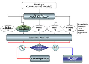
Evaluating bioavailability to aquatic invertebrates and fish can range from relatively simple tools and measures to those that are complex and integrate bioavailability factors into fate and transport models. Figure 5-1 is a generalized flow diagram that could be used to assess bioavailability and effects to aquatic invertebrate and fish communities. Methods used in these evaluations include the following:

• chemical tests
  • sediment
  • surface- or pore-water quality chemistry
  • tissue residue analyses
• biological tests
  • toxicity testing
  • population (community) surveys
• predictive
  • estimates of uptake from mathematical modeling

The major classes of these measures discussed in Chapter 4 are also germane here.

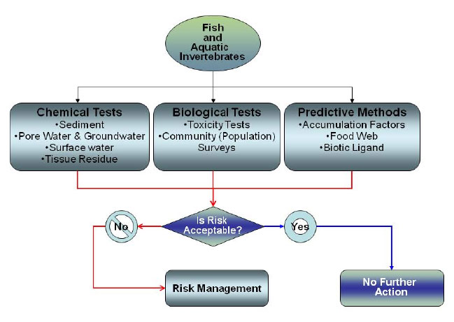Figure 5-1. Water-column invertebrate exposure evaluation for bioavailability.

Table 5-1
Tools and measures for the fish and water-column invertebrate pathway

5.2.1 Chemical Approaches
Figure 5-2 illustrates the importance of chemical measures through the food chain to fish. This illustration presents concentrations of PCB congener #52 through a Great Lakes food web to trout and salmon to demonstrate the importance of evaluating bioaccumulation from sediments and water. In this example, PCB #52 was bioavailable, at some level, in the water column and sediment. It is unclear, however, how PCB #52 became bioavailable in the water column and what fraction was bioavailable in the sediments.

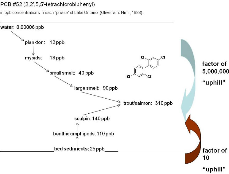
Figure 5-2. Representation of bioaccumulation pathways for PCB congener #52 in a Great Lakes food chain.
(Source: Gschwend 2008)

5.2.1.1 Sediment quality
The measures of sediment quality discussed in Chapter 4 are equally applicable for amphibians and benthic-feeding fish. While bulk sediment chemical measures are not a measure of bioavailability when correlated with biological observations such as incidence of fish tumors or lesions (Bauman et al. 1991; Bauman, Smith, and Metcalfe 1996; Meador et al. 1995; Cormier et al. 2002) or abnormal development in amphibians (Burger and Snodgrass 2000), they can be used to infer bioavailability and exposure. Statistical correlations between contaminant levels measured in sediments to those measured in fish or to incidences of observed effects are often confounded by the fact that many fish species have large home ranges and are influenced by many types of stressors. Nevertheless, bulk measures of contaminants in sediments can form the foundation for exploring those relationships.

Broader analysis of individual PCBs and PAHs is increasingly being used to characterize exposure and risks. Many site characterizations have relied on measures of Aroclors (or the sum of Aroclors as total PCBs) to characterize exposure and risk to human and ecological receptors. Measurements on PAHs may also be differentially grouped (e.g., “parent” PAHs, with sums of the low-molecular-weight PAHs [LPAHs], high-molecular-weight PAHs [HPAHs], and total PAHs) and have traditionally been used for characterization. Recent focus has been placed on using more complete bulk sediment (as well as water and tissue) analyses of the full suite of 209 PCB congeners (Cleverly 2005, California EPA 2003, DeGrandchamp and Barron 2005, NAVFAC 2001) and the parent plus 34 alkylated PAHs (Burgess 2007; Di Toro and McGrath 2000; Di Toro, McGrath, and Hansen 2000).

While these extended measures may be relevant to assessing risk at a site, there is a shortfall in the understanding of the bioavailability of each compound in the extended analyses to support risk management use. For example, there are 209 PCB congeners which do not necessarily track from sediments through a food web. While PAHs may be metabolized by fish and amphibians, they are not typically detected in tissue. Differential accumulation of PCB congeners for different species is well documented (Bright, Grundy, and Reimer 1995; Froese et al. 1998; Kay et al. 2005). Patterns of PCB congener tissue residues vary with species, trophic levels, and season. An issue paper for the Navy on PCB congeners in ecological risk assessment (NAVFAC 2001) noted that while congener-specific analyses generally offer lower detection limits and a higher information content than do Aroclor analyses, these improvements must be balanced against cost.

5.2.1.2 Water quality measures
Water quality measures have increased importance for water-column organisms. Phytoplankton and zooplankton both adsorb and absorb COPCs, which subsequently move through a food web. Amphibians absorb some chemicals across their skin. Fish can accumulate high body burdens of lipid-soluble contaminants during respiration across the gills. The physiological processes associated with chemical bioavailability across gills or skin tissue are beyond the scope of this document; however, an in-depth review is provided in a chapter by Erickson et al. (2008).

Similar to sediments, bioavailability to water-column organisms is based on the portion of a chemical that is freely dissolved. Nonionic organic compounds and some cationic metals complex with DOC and are thus not available for sorption across cell membranes in phytoplankton or across fish gills. For example, the presence of DOC binds metals such as silver, lead, copper, cadmium, and cobalt, thus reducing bioavailability to fish. Conversely, the presence of DOC may increase the bioavailability of mercury to both phytoplankton and fish. Equilibrium processes also occur in water, with contaminants partitioning between DOC, particulate OC, and the freely dissolved phases.

In addition to DOC, another factor affecting bioavailability of metals to water-column organisms is the formation of inorganic complexes, or ligands, in hard water. USEPA (2003a) defines a ligand as a “complexing chemical (ion, molecule, or molecular group) that interacts with a metal to form a larger complex.” Cationic metals such as cadmium, chromium, copper, lead, nickel, silver, and zinc are thought to form complexes with hydroxides and/or carbonates that are indicated by increased levels of calcium and magnesium (measured as “hardness”), pH, and total alkalinity. Increased hardness has been associated with decreased toxicity (and implicitly decreased bioavailability), and for these cationic metals, the associated alternate water quality criteria for freshwater may be adjusted based on measured hardness in the site water. Most states allow hardness adjustments in the calculation of water quality criteria for applicable metals. Recent research (Erickson et al. 2008), however, indicates that hardness alone cannot account for free metal ion activity, which has led to the development of the biotic ligand model (Di Toro et al. 2001, USEPA 2003a) (see Section 4.1.3.4)

Measuring the proportion of freely dissolved metals or nonionic organic compounds is still a developing science. Not all compounds are detectable in water at low levels, and it may not be possible to obtain the specificity needed for the distinction between chemical species required to assess the bioavailable fraction. Advanced analytical techniques to obtain this information may be prohibitively expensive. Traditionally, the method used to distinguish the total from the dissolved fraction of a chemical in water has been to pass the water through a 0.45 µm filter. However, a large body of evidence has demonstrated that filtration is not sufficient to separate the particulate OC or DOC from the dissolved phase, and thus the resulting filtrate may not be a suitable measure of the dissolved component in water (Nollet 2007, Boethlin and Mackay 2000).

Section 4.1.1.3 includes tools for assessing bioavailability in surface waters, and Table 2-1 provides links to information on water quality sampling and characterization. Passive samplers can provide some measure of freely dissolved compounds, but analytical detection limits and chemical speciation (e.g., metals) for some contaminants remain an issue. To minimize uncertainty with the water measures, it is important that (1) the appropriate sampler is being used, (2) the time to equilibrium is confirmed, and (3) materials have been adequately calibrated against known standards.

Luthy (2010) reports that the different polymer materials used for measurements of organic compounds by passive samplers dictate the individual properties of each sampler and thus differences in uptake rates as well as ease of application in the field. Luthy cites Adams et al. (2007) in reporting that PE is a practical material with faster time to equilibrium and less fouling than with SPMDs since only a single layer of plastic is exposed on both sides. Cornelissen et al. (2008) compared five passive samplers and concluded that the selection of a specific passive sampler depends on the objective of the study. If fast equilibrium and low detection limits are required, a thin (55 mm) POM is advantageous and has a greater chemical capacity compared to other thin samplers like SPME fibers. However, if low detection limits are not required and measurements need to be made quickly, either PE, SPME fibers, or thin POM can be used (Luthy 2010). For organic compounds, the use of performance reference compounds embedded on the sampler is needed to ascertain that the sampler is in equilibrium with the surrounding water or pore water (Fernandez, Harvey, and Gschwend 2009). Gschwend et al. (in press) compared measures made by PE, POM, and SPME of PCB congeners against direct (instrument) readings from pore water. The results in this controlled group was within a factor of 2.

5.2.1.3 Tissue residue
Measuring chemical concentrations in fish is the most common method for inferring that a specific contaminant is bioavailable. Tissue residue concentrations integrate chemical bioavailability, multiple routes of exposure, and assimilation into an organism. As discussed previously, tissue residues, coupled with bulk sediment measures, have been correlated to observed toxic effects in the field such as lesions, tumors, or subcellular effects.

Assessing bioavailability of contaminants from sediment using fish tissue residues must consider the site location, history, and size; contaminant transport processes; and the physiology, life history, size, sex, and trophic level of the target fish species. For example, for a small site with a limited area of contamination, one should consider evaluating a species with a limited home range. For larger sites, sampling could include longer trawls or multiple collections within the contaminated area. Strategies include analysis of individual whole fish, removing fillet and then separately analyzing both the fillet and offal, fish tissue plugs, compositing multiple small fish into a single analysis, or sampling from specific organs. A useful resource for considering methods of fish sampling is Assessing Chemical Contaminant Data for Use in Fish Advisories, Volume 1, Fish Sampling and Analysis (USEPA’s (2000c). This guidance provides suggested species selection criteria for fish, turtles, and shellfish; field sampling procedures (sampling design, sample collection, and sample handling); laboratory processing procedures; and analytical guidance. Other useful information in this guidance includes statistical methods given various assumptions (e.g., how many individuals per composite sample, how many replicates per composite sample).

Care must be exercised to collect the right tissue type (whole body is typically most relevant for wildlife in ecological risk assessments) and size class for an avian receptor of interest. For example, the 10–30 cm long fish generally consumed by an osprey are larger than fish (generally <20 cm long) consumed by great blue herons (Sample and Suter 1999). Tissue residues for many bioaccumulative chemicals, particularly those that biomagnify in food chains, tend to be higher in larger fish relative to smaller fish, so collecting the proper size class is an important consideration. Species of fish (or at least a guild, such as bottom feeders) must also be considered, since there may be large differences in the rate of uptake and accumulation among the various components of the fish community. Target collection must be tailored to the receptor(s) being evaluated and to the composition (relative abundance) of the fish community at the site. If concurrent chemical concentrations in sediment are measured, site-specific BAF/BSAF values may be calculated and extrapolated to other portions of the site for which tissue samples were not collected, assuming sediment contamination is an issue in these areas.

Lipid content may vary seasonally and influence bioavailability and exposures. Some species may store contaminants in fat reserves when preparing for migration, hibernation, or reproduction. Adverse effects from these contaminants may not occur until the fat reserves are metabolized for energy requirements, at which point the organism and/or its offspring may no longer be exposed to site contaminants. Lipid normalization of contaminant levels in tissue is standard practice for many organic contaminants (i.e., a factor in derivation of BSAFs) and is intended to reduce observed variability in tissue contaminant concentrations. However, the analysis of lipid(s) is not an exact science. Seasonal variation in organism lipid content and/or method variability and a lack of precision in lipid concentrations reported in units of percent can have a large impact on lipid-normalized concentrations of bioaccumulative chemicals such as PCBs and polychlorinated dibenzodioxins (PCDDs)/polychlorinated dibenzofurans (PCDFs). Typically, lipids cannot be detected in tissues below concentrations of 0.2%. Various methods (e.g., gravimetric, thin-layer chromatography [TLC]/flame ionization detector [FID]) used to determine lipid content include the use of extraction solvents (e.g., hexane, ether, chloroform) and extraction techniques (e.g., Soxhlet, accelerated solvent extraction [ASE], supercritical fluid extraction [SFE]). There is no accepted standard method (Duncan et al. 2007b). Sometimes lipid analytical methods are specified as part of a protocol for a specific contaminant such as PCBs and PCDDs/PCDFs (e.g., USEPA Methods 1668A and 1613B, respectively).

Normalization of nonionic organic contaminant sediment concentrations to the foc in the sediment is applied to the denominator of the BSAF equation. Like partitioning to lipids, partitioning to foc usually makes nonionic organic COPCs less bioavailable. While analytical methods for TOC are more established than those for lipids, analytical precision and variability in analysis of OC also can have a large impact on normalized concentrations of chemicals expressed in units of parts per trillion.

Measuring PAHs in fish tissues is not a useful measure of exposure as fish readily metabolize PAHs (Meador et al. 1995; Johnson, Collier, and Stein 2002; Johnson et al. 2008). Exposure to PAHs in fish requires measuring the metabolized PAHs in bile. Measures of biliary PAHs should be considered as estimates; the methods cannot provide a direct level of PAH concentrations in tissues. However, these measures have been correlated with other indicators of exposure and toxicity (Meador et al. 1995; Pickney et al. 2001, 2004), with one study demonstrating a positive correlation between measures of PAHs collected with a SPMD with biliary PAHs (Verweij et al. 2004). Once measured, a way of interpreting the data is via the application of the tissue residue toxicity approach (Beckvar, Dillon, and Read 2005; Dillon, Beckvar, and Kern 2010; Meador et al. 2008). Measured tissue residue values in the fish are compared to levels known to cause an acute or chronic response. One of the most commonly referenced databases in past investigations is USACE’s Environmental Residue Effects Database (ERED). While initially focused on associating adverse effects with known tissue levels, ERED has incorporated bioaccumulation data. As stated by USACE and USEPA, ERED was developed to reduce the level of uncertainty associated with interpreting bioaccumulation data for the purpose of making regulatory decisions. ERED contains tissue effects data for a wide range of species, including benthic infauna, fish, shellfish, birds, and mammals.

5.2.2 Biological Methods
Biological methods for analyzing water-column organisms are similar to those discussed for sediments and include bioassays and population surveys. While bioassays and laboratory bioaccumulation studies for fish are commonly employed for assessing contaminated sites, population surveys for fish are less frequent, due in part to the logistics associated with collecting the organisms in a systematic and statistically meaningful way. Arguably, population surveys do not provide a measure of bioavailability, but when applied in conjunction with sediment and water chemistry, bioassays, and tissue residue studies, they can help provide the links between contaminant bioavailability and effects.

5.2.2.1 Toxicity testing
Section 4.1.2.1 discussed toxicity test procedures, organisms, and interpretation in depth. Appendix C-T3 lists the standard tests.

For freshwater systems, the more commonly used aqueous-phase toxicity tests evaluate pore water, elutriates, and water-column samples. Numerous aquatic invertebrate and fish species can be used for aqueous-phase testing; method documents typically list the test species appropriate for use in the method. Other methods or species/endpoints of potential use include in situ bioassays that evaluate fish embryo development (ODEQ 2000) and tests that use amphibians (see Appendix C-T3). Commonly employed marine and estuarine toxicity tests for water-column organisms include larval bivalve tests (e.g., Mytilus, Crassostrea, Mya), mummichog (Fundulus sp.), sheepshead minnow (Cyprinidon variegates), and silversides (Menidia sp.).

5.2.2.2 Population surveys
Population surveys of fish or amphibian communities can be an important component in a weight-of-evidence approach for assessing effects. While not a direct measure of bioavailability of a contaminant, changes in characteristics of a population exposed to a site COPC imply that the contaminant is bioavailable. When coupled with other measures such as sediment chemistry, tissue residues, bioassays with the contaminated sediments or site water, suborganismal bioindicators such as lesions or tumors, or single-chemical toxicity tests, population surveys can provide a clear link between in-place contaminants, uptake, and effects (Suter et al. 1999).

How to conduct population surveys of fish or amphibians is beyond the scope of this document. A limited set of references follows, but most states have their own programs for collecting fish species associated with monitoring biological integrity of state waters or collecting samples for fish consumption advisories. More instructive is how population surveys have been used in assessments of contaminant bioavailability and risk characterization.

• Environment Canada. 1998. Fish and Fish Habitat Survey Toolkits. Victoria, B.C.: British Columbia Ministry of Environment.

• Klemm, D. J., Q. J. Stober, and J. M. Lazorchak. 1993. Fish Field and Laboratory Methods for Evaluating the Biological Integrity of Surface Waters. EPA/600/R-92/111. Cincinnati: U.S. Environmental Protection Agency, Environmental Systems Laboratory. https://projects.itrcweb.org/contseds-bioavailability/References/30002NDL.pdf.

• Meador, M. R., T. F. Cuffney, and M. E. Gurtz. 1993. Methods for Sampling Fish Communities as Part of the National Water-Quality Assessment Program. Open-File Report 93-104. Raleigh, N.C.: U.S. Geological Survey. http://water.usgs.gov/nawqa/protocols/OFR-93-104/.

• NAVFAC (Naval Facilities Engineering Command). 2004. Development of a Standardized Approach for Assessing Potential Risks to Amphibians Exposed to Sediments and Hydric Soils. TR-2245-ENV. https://projects.itrcweb.org/contseds-bioavailability/References/TR-2245-ENV.pdf.

• OEPA (Ohio Environmental Protection Agency). 2009. Fish Collection Guidance Manual Final. http://www.epa.state.oh.us/portals/35/fishadvisory/FishCollectionGuidanceManual09.pdf.

• PDEP (Pennsylvania Department of Environmental Protection). n.d. “Water Standards and Facility Regulation.” Search for “Fish Tissue Sampling and Assessment Protocol.” www.depweb.state.pa.us/portal/server.pt/community/drinking_water_and_facility_regulation/10535.

• USEPA (U.S. Environmental Protection Agency). 1994b. “Field Studies for Ecological Risk Assessment,” ECO Update 2(3). Publication 9345.0-051. Washington, D.C.: Office of Solid Waste and Emergency Response. www.epa.gov/oswer/riskassessment/ecoup/pdf/v2no3.pdf.

• USEPA. 2000c. Guidance for Assessing Chemical Contaminant Data for Use in Fish Advisories, Vol. 1: Fish Sampling and Analysis, 3rd ed.EPA/823/B-00/007. Washington, D.C.: Office of Water. http://water.epa.gov/scitech/swguidance/fishshellfish/techguidance/risk/upload/2009_04_23_fish_advice_volume1_v1cover.pdf.

• USEPA. 2002a. Clinch and Powell Valley Watershed Ecological Risk Assessment. EPA/600/R-01/050. Washington, D.C.: National Center for Environmental Assessment. http://cfpub2.epa.gov/ncea/cfm/recordisplay.cfm?deid=15219#Download.

• USEPA. 2004a. Ecological Risk Assessment for General Electric(GE)/Housatonic River Site, Rest of River. Boston: New England Region. https://projects.itrcweb.org/contseds-bioavailability/References/215498_ERA_FNL_TOC_MasterCD.pdf.

• USFWS (U.S. Fish and Wildlife Service). n.d. “Amphibian Declines and Deformities.” www.fws.gov/contaminants/Issues/Amphibians.cfm.

5.2.3 Predictive Measures
Predictive measures for identifying contaminant uptake in fish are mathematical algorithms that link sediment contaminant concentrations to residues in fish tissue. These expressions range from relatively simple ratios of contaminant concentrations in sediment or water to those in fish tissues to complex models that include transfer between trophic levels incorporating feeding rates and prey preferences; area use; assimilation efficiency; and loss by metabolism, growth, or reproduction. Bioavailability (at least to fish) is assumed in these models; the simple transfer ratios are derived from either large databases or from site-specific sediment and tissue data. The fugacity and kinetic models that are discussed are rooted in direct measures of individual uptake and loss parameters.

These models have assumed increased importance not only in assessing risk, but also in setting cleanup criteria (Glaser and Bridges 2007). Many of these mathematical equations may be rearranged to solve for sediment concentrations that are safe for human or ecological receptors. An important caution when using models is articulated in the Models in Environmental Regulatory Decision Making (NRC 2007), which indicates that models may “best be viewed as tools to help inform decisions rather than as machines to generate truth or make decisions.”

5.2.3.1 Accumulation factors
Accumulation factors for aquatic organisms are simple mathematical ratios that relate the measured concentration for a given compound in an organism (or organism compartment such as lipids) to the concentration in the medium from which the compound is taken up (Schwarzenbach, Gschwend, and Imboden 2003). Often application of accumulation factors assumes (1) all measured uptake exposure comes from a single medium (water, sediment, or prey), (2) 100% of the exposure related by the tissue measure occurs in the vicinity where that medium measure was taken, (3) the trophic level of the fish is not considered, and (d) the ratio reflects exposure to the bioavailable fraction of the contaminant in the medium.

Application of accumulation factors is widespread; they are used in the development of NRWQC (USEPA 1995a, 2000c), development of sediment protective standards in some state programs (e.g., ODEQ 2007), and prediction (internationally) of bioaccumulation into the food web (Environment Canada 1998). Despite the limits imposed by the assumptions listed above, accumulation factors for persistent and bioaccumulative organic compounds have been demonstrated to have a reasonable level of accuracy in predicting concentrations of these compounds in fish (Arnot and Gobas 2006; Burkhard, Cook, and Lukasewycz 2005; Wong, Capel, and Nowell 2001). Conversely, accumulation factors have been less reliable for metals and organo-metalloid complexes (Luoma and Rainbow 2005), which has led to the development of alternative predictive models such as the BLM (see Section 4.1.3.4, Di Toro et al. 2001). A good compilation of bioaccumulation databases is found in Weisbrod et al. (2007).

The most commonly applied accumulation factors are as follows:

• bioconcentration factor (BCF)
• bioaccumulation factor (BAF)
• biotic sediment accumulation factor (BSAF)
• biomagnification factor (BMF)

Section 5.3 discusses examples of the application of various bioaccumulation factors in remedial decision making.

BCF is the ratio of a contaminant retained in an aquatic organism following its absorption through respiratory and dermal surfaces from the surrounding water, but it does not does not include accumulation via dietary exposure (Weisbrod et al. 2007). BCFs are typically determined from laboratory bioconcentration studies. Mathematically, this is simply expressed as the concentration in tissue (mg/kg) divided by the concentration (mg/kg) in water as follows:

BAF is net uptake and retention of a chemical in an organism from all routes of exposure (diet, dermal, respiratory) and any source (water, sediment, food) as typically occurs in the natural environment (Spacie, Mccarty, and Rand 1995). Bioaccumulation typically is based on field measurements and may be expressed as either a BAF relative to freely dissolved contaminants concentrations in water or a BSAF relative to chemical concentrations in sediment (Spacie, Mccarty, and Rand 1995). Simply put, a BAF is expressed as the ratio of the concentration in tissue (mg/kg) to the concentration in sediment (mg/kg) as follows:

BSAF is used principally for estimating uptake from sediment. The estimate of the concentration on a lipid basis in fish is proportional to the concentration of a compound normalized to the sediment OC concentration. Mathematically, this relationship is expressed as follows:

where the concentration in tissue is normalized to the fraction of tissue lipids (flipid) and the dry weight sediment concentration is normalized to the foc in sediment.

BMF is used to express how the concentration of a given compound in an organism increases as one examines successive trophic levels within a given food chain (see Figure 5-3). Biomagnification is generally observed for recalcitrant lipophilic compounds with high Kow but is generally not as great a concern for metals except those which can be biotransformed to organic forms (e.g., organotins, methylmercury and methyl selenide) (NRC 2003).

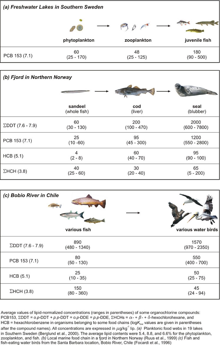
Figure 5-3. Examples of bioaccumulation and biomagnification for select organochlorines in fish-based food webs. (The legend should read µg/kg lipid or µg*kg^-1 lipid. Adapted from Schwarzenbach, Gschwend, and Imboden 2003.)

Figure 5-4. Representation of a food web used for bioaccumulation modeling.

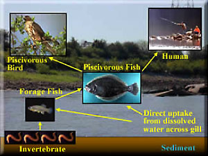
Figure 5-3 shows an example of the importance of biomagnification. Typically, within aquatic food webs BMFs are relatively small, a factor of 1–10 but generally in the range of 2–5. BMFs for higher trophic levels like birds or seals can be orders of magnitude higher. Section 5.3 discusses the application of these accumulation factors in remedial decision making. Chapter 6 covers contaminant uptake and food chain transfer to birds and mammals.

5.2.3.2 Food-web models for persistent bioaccumulative compounds
Food-web models (Figure 5-4) are an important tool for estimating the concentrations of contaminants moving from sediment into fish via the food chain. These models are applied not only in environmental decision making at contaminated sediment sites but also in setting water quality criteria, developing waste-load allocations, and evaluating new chemical products. Food-web or food-chain models have been used at a variety of sites, including the Hudson River, N.Y.; the Housatonic River, Mass.; the Lower Fox River, Wisc.; the Lower Duwamish River, Wash.; the Willamette River, Ore., Soda Lake, Wy.; and the Southern California Bight. As pointed out in Section 5.2.3, “Bioavailability (at least to fish) is assumed in these models; the simple transfer ratios are derived from either large databases or from site-specific sediment and tissue data.”

Much of the initial work in developing food-web models has been in association with PCB uptake in the Great Lakes, but more recently food-web models have also been used to estimate bioaccumulation of other nonpolar organic compounds. There are two basic classes of models for bioaccumulative compounds: fugacity and mechanistic (see Appendix C-T7). Fugacity models are steady-state mass balance equations that partition compounds through the system based on chemical properties (Mackay 1979, 1982, 1991; Campfens and Mackay 1997; Sharpe and Mackay 2000, Morrison et al. 1996, 1997). Mechanistic models are based on a series of differential equations that incorporate an array of physical and biologically based parameters, including chemical partitioning and release; uptake with consideration of feeding rates and prey preferences; area use; assimilation efficiency; and loss by metabolism, growth, or reproduction (Thoman and Connolly 1984; Thoman 1989; Thoman, Connolly, and Parkerton 1992; Gobas and Mackay 1987; Gobas 1993; Arnot and Gobas 2006, Morrison et al. 1996, 1997).

Appendix C-T5 lists several of the more commonly used bioaccumulation models. It is recommended that these models be used only with the aid of a team of modelers, statisticians, and biologists who can contribute to the parameterization and validation of the model for the specific aquatic system under consideration.

5.2.3.3 Biotic ligand model
The BLM (Figure 5-5, Appendix C-T4), discussed in Section 4.1.3.4, is especially important to the understanding of metals bioavailability to water-column organisms. A “biotic ligand” is a complexing chemical that is a component of an organism (e.g., chemical site on a fish gill) (USEPA 2007a).

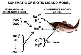Figure 5-5. Schematic of the biotic ligand model. (Courtesy HydroQual.)

Figure 5-5 shows that the model evaluates the formation of metal complexes, as well as the competitive binding at the gill interface, to determine metal toxicity. The BLM is constructed so that metal toxicity can be predicted based on the inputs of total metal concentration, temperature, pH, DOC, major cations (Ca, Mg, Na, and K), major anions (SO4 and Cl), alkalinity, and sulfide. Figure 5-6 shows that measured and BLM-predicted silver LC50 concentrations (the concentration of a chemical the kills 50% of the test species) for two species of fish and three species of Daphnia show a high degree of correlation.

A Windows version of the BLM in a simple-to-use spreadsheet format can be downloaded at www.hydroqual.com/wr_blm.html. The current version allows for calculating cadmium, copper, silver. and zinc toxicity to fathead minnows, rainbow trout, and three species of Daphnia sp.

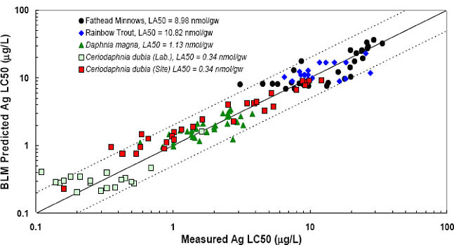Figure 5-6. Comparison of measured vs. BLM-predicted LC50 values for silver. (Source: USEPA 2007a)

5.3 Application of Bioavailability Tools in Risk Assessment and Risk Management
Contaminant levels in fish tissue are often the determining factor in setting remediation management and cleanup goals for sediment sites and most often for human health–related risks. For risk characterization specific to fish, the measured or model-estimated tissue concentrations may be compared to chemical-specific, tissue residue toxicity concentrations to determine whether the fish or amphibians are at risk from contaminant exposure. Bioassays or population surveys can provide an additional line of evidence to the assessment of potential risks to the fish or amphibian communities. However, as the case studies below illustrate, a commonly observed condition is that site chemical data stands in direct contrast to population surveys or bioassays. Best professional judgment is required to sort through the data to determine the risk management action.

Remedial action levels in sediments can be set by determining an acceptable level of risk based on tissue residues and using the mathematical factors or models discussed in Section 5.2.3 in reverse to solve for the “safe” sediment concentrations. An example of this process is the Oregon SQGs derived for fish consumption discussed in Chapter 2, where the safe tissue residue values for human consumption are determined and BSAFs are used to back-calculate the presumed safe sediment value. This practice, however, typically results in very conservative sediment concentrations (often below naturally occurring background levels).

The same four principal areas discussed in Section 4.2, where bioavailability data may be applied to inform decisions and remedies, risk assessment, risk management, remedial selection, and remedial design/implementation, are equally applicable here. Appendix D contains details of each of the case studies cited below.

5.3.1 Bioavailability in Risk Management
For water-column organisms, assessment of bioavailability can have a critical role in the following three risk management objectives:

• identification of appropriate stressor(s)
• identification of exposure route(s)
• development of sediment cleanup levels

USEPA’s general guidance document for the identification of stressors (USEPA 2000c), in conjunction with the TIE procedures of USEPA (Burgess et al. 1996; USEPA 1989b, 1989c) and/or states (e.g., California EPA 2008), are applicable to water-column invertebrates and fish.

Stressor Identification
Identifying stressors for water-column organisms can follow the same general principles previously outlined in Section 4.2.1 Efroymson et al. (1996) provided a series of questions that should be considered to determine where contaminants are bioavailable:

• Is the fish community less species rich or abundant than would be expected?
• Do individual fish display injuries that are indicative of significant toxic effects?
• Is the water toxic to aquatic organisms?
• Does the water contain chemicals in toxic amounts?
• Do the fish contain chemicals in toxic amounts?
• What factors account for apparent discrepancies in the results?
• What is the likelihood that the fish community is at least 20% less species rich or abundant than it would be in the absence of contamination?

It should be noted that investigations of aquatic community stressors may not always yield a clear conclusion. For example, Suter et al. (1999) noted that, for the Clinch River OU in Tennessee, only one of the subareas offered a clear relationship upon which remedy decisions could be made. For the Spring River in Kansas, a clear correlation could be demonstrated between metal concentrations and aquatic community impacts. Conversely, at a former wood-treating facility in Oregon, there were no connections to site contaminants, which suggested that the contaminants were not bioavailable or that measured endpoints were not sensitive enough to detect the effects.

Tri-State Mining District, Spring River and Tributaries, Kansas, Missouri, and Oklahoma
The Tri-State Mining District (TSMD) study site provides an example of using studies that demonstrate a clear relationship between stressors in the water and effects to water-column organisms. The TSMD encompasses a large area in southeastern Kansas and adjoining portions of Missouri and Oklahoma. Commercial extraction of Pb- and Zn-bearing ores from more than 4,000 subsurface mines over 120 years left a legacy of health and environmental problems, including elevated contaminant levels in fish and probable declines in some native fish and macroinvertebrate populations. To determine whether elevated levels of selected metals in surface water and fluvial sediment were possible factors limiting the distribution and abundance of freshwater mussels in the Spring River Basin, population surveys and supporting physical habitat assessments were performed throughout the basin and above and below former mining sites. Concentrations of 16 trace elements in surface waters and tissues of mussels and Asian clams (Corbicula fluminea) were determined at most survey sites. Overall, streams draining heavily mined areas exhibited depauperate (or fully extirpated) mussel assemblages and correspondingly elevated concentrations of Cd, Pb, and Zn in water, sediment, and bivalve tissue. Other evaluated environmental chemistry parameters and physical habitat conditions assessed at the stream reach scale demonstrated little general relationship to the degraded status of these assemblages. Taken together, these results suggested that pollution attributable to former mining operations is bioavailable and continues to adversely influence environmental quality and impede the recovery of mussel communities in a large portion of the Spring River Basin.

McCormick and Baxter Superfund Site, Oregon
Fish and crayfish surveys were conducted at this former wood-treating facility on the shores of the Willamette River in Portland (Pastorok et al. 1994). To assess the effects of the residual creosote-derived contaminants including PAHs and dioxins, the assessment included sediment chemistry, bioassays, tissue residues in fish and crayfish, and fish histopathology. Sediment chemistry and toxicity testing indicated that a substantial area of the Willamette River sediments proximal to the site was likely to be toxic (USEPA 1996n). By contrast, tissue residue values for PAHs in crayfish (Pacifastacus leniusculus) and large-scale sucker (Catastomus macrocheilus) were low (PAH metabolites were not measured), and there were no statistical differences between the site and upstream in the histopathology of the 249 fish livers examined. Based principally on the sediment chemistry and bioassay data, as well as continuing NAPL discharges from sediments to the Willamette River, the ROD required the placement of an impermeable cap (USEPA 1996n).

5.3.2 Bioavailability in Remedy Selection
Bioavailability considerations in remedy selection are highlighted below. In one case, NFA was indicated. In the second, a removal will occur, with post-removal risk verification confirmed by using bioaccumulation modeling for fish. While other exposure pathways were considered for these sites, only the fish receptor pathways figured into the remedy selection.

Fifteen Mile Creek, Oregon
Approximately 2600 gallons of the pesticide oxyfluorfen (2-chloro-1-(3-ethoxy-4-nitrophenoxy)-4-(trifluoromethyl) benzene) spilled into Fifteen Mile Creek, located proximal to the Columbia River. Approximately 1200 feet of the creek from the accident site to the confluence with the Columbia River was affected. While not especially toxic to mammals or birds, the pesticide is toxic to fish. The Oregon Department of Fish and Wildlife estimated that about 5500 fish died as a result of the spill. Post-spill monitoring over a three-year period evaluated the persistence and bioavailability of oxyfluorfen. Chemical-specific measurements were performed in sediment, upland soil, surface water, pore water, and crayfish and trout. Site-specific sediment/water and biota-sediment accumulation factors were determined. Bioaccumulation in fish tissue was evaluated based on the chemical concentrations in caged trout, juvenile and adult, and crayfish. Other data included laboratory bioassays, benthic invertebrate studies, fish histopathology, and chemical concentrations in the diet of lamprey, trout, crayfish, and piscivorous mammals. Caged trout were placed in the creek for 30 days in June 2001 to evaluate their survival rate and tissue residues. These data were used to evaluate ecological risks, as well as human exposure pathways for subsistence and sport fishermen and recreational swimmers. After three years of sampling, risk assessment indicated that residual contamination did not exceed acceptable levels. Therefore, no further action was required.

Bradford Island Removal Project, Oregon
Bradford Island is part of the Bonneville Dam complex on the Columbia River approximately 40 miles east of Portland. The site is located adjacent to the former Bradford Island landfill, and the contaminants of interest (COIs) include PCBs, PAHs, and metals. An in-water removal of sediment was conducted in 2007. Following the removal action, the data indicate unacceptable levels of PCBs in crayfish and fish tissue; however, the report emphasizes that this may not be an accurate reflection of site risk because the organisms sampled were likely exposed to contamination in sediment that has since been removed. The current recommendation by USACE is to monitor tissue levels in the future when a true picture of current exposures can be obtained.

²Lists of parent PAHs vary across different federal and state programs. USEPA lists 18 parent PAHs, while many state programs list 16–18. A common set of PAHs includes naphthalene, 2-methylnaphthalene, acenaphthylene, acenaphthene, fluorene, phenanthrene, anthracene (LPAHs), fluoranthene, pyrene, benzo(a)anthracene, chrysene, benzo(b+k)fluoranthenes, benzo(a)pyrene, indeno(1,2,3-cd)pyrene, dibenzo(a,h)anthracene, and benzo(g,h,i)perylene (HPAHs).