


6.0 Bioavailability to Wildlife
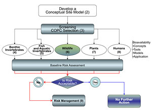
The focus of this section is how the bioavailability of contaminants in freshwater and marine sediments can be incorporated into ecological risk assessments (ERAs) of avian and mammalian wildlife receptors. Figure 6-1 shows a general flow diagram for this consideration.
Since the focus is on aquatic systems (sediments), the key avian groups of potential concern are as follows:
- omnivores (e.g., ducks, geese, swans, gulls)
- piscivores (e.g., herons, egrets, bald eagles, ospreys, kingfishers, loons, cormorants, pelicans)
- invertivores (e.g., stilts, sandpipers, rails)
- aerial insectivores that forage over/near open-water areas (e.g., swallows, terns) or wetland insectivores (e.g., marsh wrens)
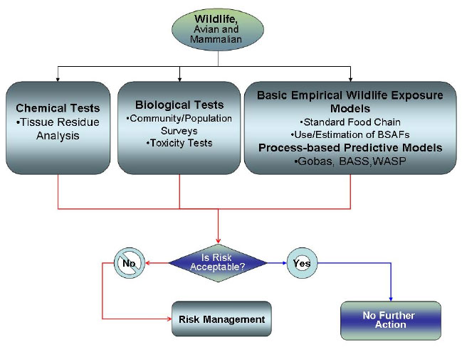 Figure 6-1. Evaluating avian and mammalian wildlife for bioavailability.
Key mammalian groups are as follows:
- aquatic and semiaquatic herbivores (e.g., beavers, muskrats)
- semiaquatic omnivores (e.g., raccoons)
- piscivores (e.g., otters, minks)
- insectivorous mammals (e.g., bats)
- marine mammals (e.g., harbor seals, sea otters)
6.1 Conceptual Site Model for Wildlife Receptors
Most wildlife exposure to environmental contaminants is from dietary intake, particularly for chemicals that bioaccumulate. Exceptions are fish and species with incidental sediment ingestion (e.g., dabbling ducks, sandpipers). Exposure from inhalation, dermal contact, and drinking water are generally insignificant relative to dietary intake and sediment ingestion.
Exposure is, thus, heavily influenced by bioaccumulation/bioavailability of contaminants in sediment/pore water to lower trophic level species (mainly fish and water-column invertebrates—Chapter 5 and plants—Chapter 7). These are prey for aquatic or semiaquatic wildlife and avian species. While there are some receptors that prey on adult birds, eggs, or young or semiaquatic mammals (such as muskrats), these receptors are the exception, and consumption of these prey species may be seasonal and/or opportunistic.
USEPA (2000a) has developed a list of chemicals that are persistent, bioaccumulative, and toxic (PBT) compounds in sediments. Table 6-1 lists suspected bioaccumulating chemicals for ecological pathways. It is not intended to be an extensive review of the literature for these target chemicals. States may have additional chemicals that expand on this list, for example Oregon (ODEQ 2007).
6.2 Chemical Approaches
Wildlife soil screening levels (SSLs), if available (for example, ODEQ 2007), can be used as a first-cut tool to determine whether contaminant concentrations in sediment are not expected to result in a risk to wildlife. These SSL concentrations are derived from empirical dietary studies with representative species in which chemical concentrations in the diet were observed to cause toxicity. The degree of bioavailability observed is specific to the study conditions and test species and may not represent site-specific conditions or species at other locations where the screening levels are applied. There are two parts to the development of wildlife SSLs:
- Determine the most appropriate endpoint and associated safety factor(s) for risk assessment. Endpoints used may include the lowest dose or concentration resulting in a NOAEL or a “lowest observable adverse effects level” (LOAEL) in a receptor.
- Relate the results for the test organism to the site conditions and target species of interest and the sediment concentrations of the COI.
Table 6-1
Table 6-1. Chemicals of concern (Source: USEPA 2000a)
List 1 (Required for Analysis) |
List 2 (Strong Concern and Priority for Study) |
|||||
| Chemical | Analytical method | Chemical | Analytical method | |||
| Metals (mg/kg) | Metals (mg/kg) | |||||
| Arsenic | 6020 | Chromium VI | 7196A or 7199 | |||
| Cadmium | 6020 | Polycyclic aromatic hydrocarbons (µg/kg) | ||||
| Chromium | 6020 | Benzo(a)pyrene | 8270C | |||
| Copper | 6020 | Biphenyl | 8270C | |||
| Lead | 6020 | Perylene | 8270C | |||
| Mercury | 7471A | Halogenated extractable compounds (µg/kg) | ||||
| Nickel | 6020 | 1,2,4,5-Tetrachlorobenzene | 8270C | |||
| Selenium | 7740 | Heptachoronaphthalene | 8270C | |||
| Silver | 6020 | Hexachloronaphthalene | 8270C | |||
| Zinc | 6020 | Octachloronaphthalene | 8270C | |||
| Polycyclic aromatic hydrocarbons (µg/kg) | Pentabromodiphenyl ether | 8270C | ||||
| Fluoranthene | 8720 | Pentachloronaphthalene | 8270C | |||
| Pyrene | 8720 | Tetrachloronaphthalene | 8270C | |||
| Chlorinated aromatics (µg/kg) | Tetraethyltin | Michelsen, Shaw, and Stirling 1996 | ||||
| Hexachlorobenzene | 8081A | Trichloronaphthalene | 8270C | |||
| Phenols (µg/kg) | Miscellaneous extractables (µg/kg) | |||||
| Pentachlorophenol | 8270 | 4-Nonylphenol, branched | 8270C | |||
| Pesticides and PCBs (µg/kg) | Pesticides (µg/kg) | |||||
| Chlordane | 081A | Chlorpyrifos | 8141 | |||
| Alpha-benzene hexachloride | Dacthal | 8081A | ||||
| Total Aroclor PCBs | 8082 | Diazinon | 8141 | |||
| Total DDT | 8081A | Endosulfan | 8081A | |||
| Ethion | 8141 | |||||
| Kelthane | 8081A | |||||
| Mirex | 8081A | |||||
| Oxadiazon | 8141 | |||||
| Parathion | 8141 | |||||
| Trifluralin | 8081A | |||||
Unless assuming a direct (incidental) ingestion of sediment in the diet (e.g., sandpipers), relating chemical concentrations in sediments to an anticipated exposure scenario for a receptor can be difficult since the association often depends on an indirect relationship between the diet and the site-specific sediment concentrations. Some regional and state approaches for these evaluations are listed below. Some of the approaches provide useful information for deriving wildlife SSLs but may require additional modeling, conservative assumptions, or other information to create SSLs that are relevant to wildlife inhabiting or foraging at the site.
USEPA
USEPA (U.S. Environmental Protection Agency). 1993. Wildlife Exposure Factors Handbook, 2 vols. EPA/600/R-93/187. Washington, D.C.: Office of Research and Development. http://cfpub.epa.gov/ncea/cfm/wefh.cfm?ActType=default.
State Guidance
-
NJDEP (New Jersey Department of Environmental Protection). 1998. Guidance for Sediment Quality Evaluations. http://www.nj.gov/dep/srp/guidance/srra/ecological_evaluation.pdf.
-
ODEQ (Oregon Division of Environmental Quality). 2007. Guidance for Assessing Bioaccumulative Chemicals of Concern in Sediment. Environmental Cleanup Program. https://www.oregon.gov/deq/FilterDocs/GuidanceAssessingBioaccumulative.pdf
-
OEHHA (Office of Environmental Health Hazard Assessment). n.d. “Cal/Ecotox (California Wildlife Biology, Exposure Factor, and Toxicity) Database.” California Environmental Protection Agency in collaboration with University of California at Davis.
-
WDOE (Washington Department of Ecology). 2001. “Site-Specific Terrestrial Ecological Evaluation Procedures.” Washington Administrative Code (WAC) 173-340-7493. www.ecy.wa.gov/programs/tcp/policies/terrestrial/wac_1733407493.htm.
Departments of Defense and Energy
-
NFESC (Navy Facility Engineering Service Center). 2003b. Guide for Incorporating Bioavailability Adjustments into Human Health and Ecological Risk Assessments at U.S. Navy and Marine Corps Facilities, Part 1: Overview of Metals Bioavailability. https://projects.itrcweb.org/contseds-bioavailability/References/bioavailability01.pdf.
-
Sample, B. E., and G. W. Suter II. 1994. Estimating Exposure of Terrestrial Wildlife to Contaminants. ES/ER/TM-125. Ridge, Tenn.: Oak Ridge National Laboratory. http://www.esd.ornl.gov/programs/ecorisk/documents/tm125.pdf.
-
U.S. Army Public Health Command. n.d. “Army Risk Assessment Modeling System (ARAMS).” http://phc.amedd.army.mil/topics/labsciences/tox/Pages/ARAMS.aspx.
Advantages
- Directly assesses bioaccumulation
- Can be nondestructive
- May not be expensive (e.g., feather collection)
- Can be used for multiple COCs
Disadvantages
- Can be complicated and require a high skill level (e.g., blood collection)
- Addresses only a single receptor at a time
- Direct extrapolation to effects may not be possible
Tissue Residue Analysis
Depending on the receptor tissues evaluated, analysis of chemical concentrations can provide a direct measurement of biological uptake. Many investigators have attempted to relate adverse toxicological effects in birds to the concentrations of individual COPCs in specific avian tissues (Beyer, Heinz, Redmon-Norwood 1996). The tissues most commonly investigated in birds and mammals and the associated COPCs include the following:
- eggs (metals, metalloids such as selenium, PCBs, organochlorine pesticides, PCDDs, and PCDFs)
- feathers, fur (e.g., mercury)
- blood (e.g., lead)
- organs, such as brain, kidney, and liver (metals, metalloids, PCBs, organochlorine pesticides, PCDDs, and PCDFs)
- fat/blubber (in marine mammals, lipophilic contaminants such as PCBs and polybrominated diphenyl ethers)
An advantage of testing feathers, fur, blood, body fat, or muscle is that it can be done nondestructively and the organism does not need to be sacrificed. Measures in tissues such as feathers or fur, however, are not well suited for evaluating bioaccumulation of most contaminants. Feathers and fur are typically routes for excretion and detoxification; therefore, concentrations in these tissues may not be indicative of anything except relative exposure.
Field tissue residue measurements can be compared to laboratory-derived tissue residue thresholds. These threshold values can be found in the various databases, including USACE ERED (USACE n.d. “The Environmental”); Jarvinen and Ankley (1999); Beyer, Heinz, Redmon-Norwood (1996); and the Contaminant Hazard Review series published by the U.S. Geological Survey (USGS). These databases are relevant to wildlife species as they include tissue residue values and thresholds for many bird and mammal species. Receptors contained in the above references may not be applicable to a given site. In these cases surrogate species are often used.
Unfortunately, for most chemicals, the advantage the tissue-based toxicity approach provides in reducing uncertainty in the assumptions of chemical bioavailability is offset by the additional uncertainty introduced by the development of the tissue-based toxicity reference values. Our level of understanding regarding the critical body burden and/or toxic mode of action and the amount of data which we have for chemicals like selenium, lead, and cadmium is atypical. For most chemicals, more data are available for dose-response or concentration-response relationships than for tissue residue toxicity relationships. Thus, the estimation of impacts associated with specific tissue residues remains limited by the state of the science.
6.3 Biological Approaches
An additional set of options involves collecting information on actual (direct) measures (Appendix C-T9) of impairment. These tools can be used as an adjunct or replacement for modeling and can indicate whether contaminants are bioavailable at a site. The following are some of the commonly available tools
6.3.1 Population Surveys
Population surveys are methods of evaluating abundance and reproductive success of receptors and may be used to infer the effects of exposure to COPCs. Population sampling may include measurement endpoints such as population counts and age structure, bird clutch size and fledging success, mammal pup/kit counts, and weight gains. See Section 4.1.2.2 for a description of how community structure and function can provide evidence of COPC-related effects.
6.3.2 Toxicity Testing
Toxicity tests typically measure toxic effects of contaminants on organisms under controlled conditions. While a study of this type does not directly relate the fish tissue concentration to the sediment concentration, it can account for the bioavailability and toxicity of the COPCs as they occur in the prey diet (e.g., fish) of the wildlife species used for testing. Laboratory toxicity studies can be conducted with a contaminated diet collected in the field (see below) or spiked in the laboratory or using other dosing mechanisms (e.g., oral gavage).
Advantages
- Controlled environment
- Direct relationship between tissue and sediment
Disadvantage
- Not as representative of site conditions
For an example of laboratory toxicity testing in mammals, ecological risk assessments of PCBs in the Housatonic and Saginaw rivers were conducted by collecting carp directly from these rivers, analyzing PCB concentrations in the carp, and formulating feed to obtain different dose levels for two-generation caged mink studies (Bursian and Aulerich 2003, Bursian et al. 2006, Heaton et al. 1995, Tillet et al. 1996). The mink were monitored for several effects endpoints (i.e., body weight, organ weight, behavior, reproductive success, offspring weight, offspring weight gain) that could be associated with the specific concentration of PCBs in the carp. Dose-response curves were successfully generated for both studies for several endpoints, accounting for the potential contribution of other contaminants in the fish to the observed toxicity.
6.4 Basic Empirical Wildlife Exposure Models
A variety of models and tools be applied to estimate bioavailability from sediments to biota (Appendix C-T9). These tools range from the incorporation of site-specific information into simple equations (ODEQ 2007, USEPA 1993) relating sediment concentrations to effects on wildlife species to more complicated models that incorporate an increasing number of site-specific variables into the dynamics of contaminant movement in the food chain. These tools predict tissue concentrations or adverse biological effects. At the most comprehensive level, models that include consideration of seasonal changes (e.g., diet and home range) and digestive processes (kinetic-, energetic- and fugacity-based trophic models) can be applied for assessing potential bioaccumulation and/or effects.
Advantages
- Inexpensive
- Can be performed using assumptions with a limited number of site-specific inputs
- Unlikely to underestimate exposure
- Generally accepted by regulators
- Determining data representativeness
- Requires field measurements to calibrate and obtain site-specific results
- Likely to overestimate exposure
6.4.1 Basic Modeling Inputs
At the most basic level (i.e., screening level assessments), the only site-specific inputs (other than selecting specific wildlife receptors that are relevant to a site based on habitat and other factors) to a food-web model are the measured concentrations of chemicals in water and/or sediment. Receptor-specific model inputs (food and water ingestion rates, dietary composition [including incidental sediment ingestion], and body weight) are based on available literature values (e.g., USEPA 1993). This screening-level assessment typically uses conservative estimates for these parameters and assumes 100% contaminant bioavailability. While useful for screening assessments, this assumption is often incorrect, particularly for metals in sediment that are known to have relatively low bioavailability factors (e.g., arsenic, barium, lead and chromium). If subsequent quantitative risk assessment is necessary, assumptions such as this should be refined to better reflect likely site and receptor parameters values. As previously described in Section 5.2.1.2, lower trophic level organism (prey) tissue concentrations are typically modeled from sediment (or water) using literature-based BSAFs or BAF/BSAF models (which allow for some adjustment for site-specific conditions (e.g., using measured site TOC or percent tissue lipid into the BSAF formula). Section 5.2.3.1 described accumulation factors for fish and aquatic invertebrates in more detail. Table 6-2 provides some key sources of BAF/BSAF values. ODEQ (2007), RSET (2009), and USEPA (1993) provide additional information on exposure factors relevant to wildlife tissue residue modeling based on chemical concentrations in sediment.
Animals that consume fish typically have the lowest sediment ingestion rates; species that consume bivalves, benthic invertebrates, and rooted vegetation have much higher rates (up to 22 percent for the canvasback; (Beyer et al. 2008). Benthic-feeding shorebirds may have incidental sediment ingestion rates of up to 30 percent (Beyer et al. 1994).
6.4.2 Exposure Considerations
There are differences in chemical bioavailability from ingested tissue versus ingested sediment since the disposition and form of the COPC may differ. For example, mercury and arsenic in sediment are typically present as inorganic forms, but fish tissue contains almost entirely methylated organic forms of these metals. Living organisms metabolize many organic chemicals, so prey tissue may contain metabolites as well as the parent compounds. Some of these metabolites may be more toxic than the parent compound (e.g., PAHs, dichlorodiphenyldichloroethene [DDE]). DDE, a metabolite of dichlorodiphenyltrichloroethene (DDT), is generally considered more toxic for reproductive effects than the parent compound. Metabolites may not be present in sediment unless physical, microbial, or other biological processes change the chemical form of the parent compound. In addition, for chemicals like PCBs, PCDDs, and PCDFs, certain congeners tend to be degraded or metabolized at slower rates than others, leading to a relative enrichment of particular congeners in both sediment and the associated food web over time. Thus, the congener distribution in a sediment sample will likely differ from that in a plant sample, which will differ from that in a fish or bird tissue sample. This variability complicates modeling of bioaccumulation through the food web.
Some site assessments have made simplifying assumptions based on the availability of the contaminants as a result of the physical characteristics of the habitat (e.g., depth of water, depth of bioturbation zone). In general, avian and mammalian species limit their foraging to water depths of 25 feet or less. For example, double-crested cormorants dive from the water surface to an average depth of 15 feet and a maximum depth of 26 feet (Johnsgard 1993). Eelgrass, which is a principal dietary component for many bird species, occurs at depths only up to 25 feet in Puget Sound (Washington Department of Natural Resources 2001). While mammals such as harbor seals and river otters may dive to deeper depths, most of their foraging activity is likely to be in the upper meters of the water column where prey species are most abundant and their visual-based ambush strategy is more effective (USEPA 1993).
As discussed previously, most ERAs use “standard” food-web models to estimate exposure to wildlife from dietary pathways. Bioavailability should be accounted for in the estimate or measurement of the dietary sources, as well as the fraction of the contaminant present in the food source that is assimilated by the receptor. Thus, the next step in making the model more representative of site conditions is the incorporation of site-specific concentrations.
6.4.3 Site-Specific Measurements
Given the uncertainties with non-site-specific BSAFs (see Section 4.1.3.3), direct sampling of prey tissues is the most robust quantitative measure of bioaccumulation and bioavailability. Direct tissue measurements integrate bioavailability directly into the methodology and allow calculation of site-specific BSAFs (Meador et al. 2008). These BSAFs can then be extrapolated to the universe of dietary sources and receptors.
BSAF determinations have implicit sources of uncertainty and variability built in, including the following, each of which is clarified below:
- lipid analysis
- OC analyses and sediment foc
- chemical analysis of contaminant concentrations in organism tissues
- identification of appropriate site-specific factors linking the organism to the sediment
Lipid content, in both prey and the wildlife receptors, may vary seasonally and influence bioavailability and exposures. Some species may store contaminants in fat reserves when preparing for migration, hibernation, or reproduction. Adverse effects from these contaminants may not occur until the fat reserves are metabolized for energy requirements, at which point the organism and/or their offspring may no longer be exposed to site contaminants. Lipid normalization of contaminant levels in tissue is standard practice for many organic contaminants (i.e., a factor in derivation of BSAFs) and is intended to reduce observed variability in tissue contaminant concentrations. However, the analysis of lipid(s) is not an exact science. Seasonal variation in organism lipid content and/or method variability and a lack of precision in lipid concentrations reported in units of percent can have a large impact on lipid-normalized concentrations of bioaccumulative chemicals such as PCBs and PCDDs/PCDFs. Typically, lipids cannot be detected in tissues below concentrations of 0.2%. Various methods (e.g., gravimetric, TLC/FID) used to determine lipid content include the use of extraction solvents (e.g., hexane, ether, chloroform) and extraction techniques (e.g., Soxhlet, ASE, SFE). There is no accepted standard method (Duncan et al. 2007b). Sometimes lipid analytical methods are specified as part of a protocol for a specific contaminant such as PCBs and PCDDs/PCDFs (e.g., USEPA Methods 1668A and 1613B, respectively).
Normalization of nonionic organic contaminant sediment concentrations to foc in the sediment is applied to the denominator of the BSAF equation. Like partitioning to lipids, partitioning to foc usually makes nonionic organic COPCs less bioavailable. While analytical methods for TOC are more established than those for lipids, analytical precision and variability in analysis of OC also can have a large impact on normalized concentrations of chemicals expressed in units of parts per trillion.
for Direct Measurements
Advantages
- Controlled environment
- Direct relationship between tissue and sediment
Disadvantage
- Not as representative of site conditions
Another factor influencing variability in observed BSAF concentrations is the fact that even with sessile organisms, the ability to co-locate biota and the sediment to which the biota are exposed may be challenging. In practice, the top 10–15 cm of sediment is considered to be the biological active (or bioturbation) zone (Oliver et al. 1980, Weston 1990, Aller and Dodge 1974) and is the sediment interval that is sampled for the determination of site-specific BSAFs. However, the animals that live in or below this zone (e.g., burrowing clams, worms, shrimp), principally in marine habitats, may feed or draw in water at the sediment surface or may have feeding strategies that are selective to particle size or to suspended particulates. Therefore, the sediment contaminant concentrations to which these organisms are exposed may differ substantially from bulk sediment concentrations in the top 10–15 cm that are typically used to normalize foc.
Prey items for the vast majority of wetland and aquatic avian receptors are plants, invertebrates (including shellfish, like mollusks), and/or fish. Other prey items may include amphibians, reptiles, other birds, and small mammals, but these prey items do not typically compose a significant proportion of the diet for most wetland and aquatic avian receptors. For some site-specific baseline investigations, tissue concentrations may be measured in some prey species but not in others; therefore, modeling methods are used for those prey items that are not measured but are considered in the diet of the receptor.
Additional guidance for the direct sampling of chemical concentrations in tissue can be found in the following:
- Biomonitoring of Environmental Status and Trends (BEST) Program: Selected Methods for Monitoring Chemical Contaminants and Their Effects in Aquatic Ecosystems (Schmitt and Dethloff 2000)
- Biomonitoring of Environmental Status and Trends (BEST) Program: Field Procedures for Assessing the Exposure of Fish to Environmental Contaminants (Schmitt et al. 1999)
- Ecological Risk Assessment Guidance for Superfund: Process for Designing and Conducting Ecological Risk Assessments (USEPA 1997b)
- “Field Studies for Ecological Risk Assessment” (USEPA 1994b)
Bioaccumulation into prey species, which are consumed by wildlife species, can be evaluated using laboratory testing techniques. Laboratory bioaccumulation test methods are available on invertebrate test species (polychaetes, oligochaetes, insect larvae, bivalves, and crustaceans) (USEPA 1991, 1998b, 2002e; ASTM 2010) in both freshwater and marine environments. Other parameters required for a wildlife exposure model (e.g., site-specific receptor body weights, ingestion rates, and dietary composition) are rarely quantified on a site-specific basis. Bioaccumulation (and bioavailability) can also be evaluated by placing caged organisms (e.g., mussels) or units that mimic bioaccumulation (such as SPMDs) at the site for a predetermined time period and then analyzing the tissue or device for contaminant accumulation.
Advantages
- Can be less expensive than effects measurements
- Does not require direct evaluation of target receptors and is less intrusive than tissue sampling
- Can potentially incorporate multiple exposure mechanisms
Disadvantages
- Requires a high skill level and input from multiple disciplines to complete
- Potential for error without sufficient field validation of key model parameters
- May not be acceptable by regulators as a final result, especially if it indicates no unacceptable exposure
6.5 Process-Based Predictive Models
Predictive models (Appendix C-T9) based on kinetic, mass balance, and steady-state relationships have been developed to describe the bioaccumulation of HOCs in aquatic food webs (e.g., Thoman, Connolly, and Parkerton 1992; Gobas 1993; Arnot and Gobas 2004). The bioaccumulation portion of these models rely on the contaminants’ Kow to estimate uptake and elimination constants through respiration and diet of aquatic organisms in different trophic levels. Contaminant tissue concentrations in aquatic organisms are calculated (i.e., modeled) for different trophic levels of a food web through diet and respiration. The modeled tissues concentrations can then be used to estimate dose- and dietary-based exposure and risk quotients for upper trophic level mammals and birds consuming aquatic organisms (USEPA 2009).
Kow can influence exposure as follows:
- For chemicals with a log Kow <4, direct uptake from water is a more important exposure pathway.
- For chemicals with a log Kow >4, dietary uptake is the more important means of chemical exposure and there may be potential for food-chain transfer.
In general, these models are sensitive to chemical Kow, lipid content, and the ratio between the chemical concentration in the water column and in the sediment. These factors can be difficult to quantify since literature-based Kowws vary depending on the source used, tissue lipid analytical methods are generally not precise, and even with low limits of detection it is difficult to measure HOC concentrations in surface water. Notwithstanding the above, these models are generally accepted by the scientific community as a reasonable approach for estimating the bioaccumulation of persistent HOCs in aquatic systems (Burkhard 1998). A few of the more well-known predictive models, some of which have been applied to a variety of sites, are briefly discussed below.
The Gobas (1993) model has been used to successfully estimate concentrations in fish and wildlife, primarily for lake food webs. The Gobas (1993) model for fish is currently available in electronic format from Simon Frasier University (see Appendix C-T5, C-T7). The model is also available embedded in a forwardly predictive, risk-based program: TrophicTrace. Each of these forms of the model is restricted to fish as prey species for birds and mammals. Arnot and Gobas (2004) published a broader model that includes other aquatic species that could be prey for wildlife and mammals. Although originally developed and applied to the Great Lakes ecosystem for modeling PCBs and selected pesticides, the Arnot and Gobas (2004) model has been applied and validated for other ecosystems, including the Hudson River, Fox River/Green Bay, and Bayou D’Indie in Louisiana.
In the 1980s, USEPA initiated the Gill Exchange and Transport System (GETS) model for calculating chemical uptake into aquatic organisms. This model was amended with a food component to form the Food and Gill Exchange Transport System (FGETS) while the successor model to FGETS is the Bioaccumulation and Aquatic System Simulator (BASS) model (USEPA n.d. "Bioaccumulation"). The BASS model simulates the population and bioaccumulation dynamics of age-structured fish communities. Further information on these models can be found at www2.epa.gov/exposure-assessment-models/bass.
WASP7 (Water Quality Analysis Simulation Program) (USEPA n.d. "Water") helps users interpret and predict water quality responses to natural phenomena and man-made pollution. This revised and updated version of the WASP model is currently available in the public domain at www.epa.gov/athens/wwqtsc/html/wasp.html. This version incorporates fish age structure and population dynamics into the simulation of the bioaccumulation of hydrophobic COPCs.
Research to validate these legacy models in aquatic ecosystems has resulted in the general conclusion that the models are accurate within an order of magnitude (Burkhard 1998). Thus, many risk assessors have chosen to calibrate the models with subsequent field sampling programs or to skip the modeling activities and empirically evaluate the bioavailability of contaminants by directly sampling aquatic organisms.
6.6 Application of Bioavailability Measures in Risk Assessment and Risk Management
As discussed previously, the methods for evaluating contaminated sediment impacts on wildlife run the gamut from simple literature-based evaluations to detailed modeling and site-specific toxicity studies. As the level of complexity increases, the opportunities for accounting for the bioavailability of contaminants also increase. In many cases, several lines of evidence are evaluated to determine whether the contaminant is (1) not bioavailable to the wildlife, (2) bioavailable at levels that are unlikely to cause an adverse impact, or (3) bioavailable at levels that require remedial action. The following examples of receptor evaluations identify how the bioavailability assessment was used to quantify risk at a site
Avian Receptors (Tree Swallow)
Tree swallows are aerial insectivores that forage over wetland and aquatic habitats and are thus exposed via the diet of insects that emerge from contaminated sediments. This species is a very useful avian receptor for evaluating contaminated sediments because of the following:
-
Population Survey:They readily use nest boxes, so study areas can be established at specific locations of interest where suitable habitat is present.
Tree Swallow Example
The tree swallow is a species frequently used for site nesting evaluations, particularly for PCB- or dioxin-contaminated sites, because it nests in artificial structures and thus can be attracted to a site through the erection of such structures. Nest boxes also lower predation rates (a potential confounding factor) and allow easy access for monitoring egg laying, nestling growth, and nest success or for collecting eggs or young for tissue residue analysis. Tree swallows are aerial insectivores that forage over wetland and aquatic habitats and thus are exposed via the diet to insects that emerge from contaminated sediments. - Individual swallows generally feed within 400 m of their nest sites on emergent aquatic insects, so residues in their tissues reflect local sediment contamination for chemicals that readily accumulate in such tissues.
- Tree swallows nest within close proximity to one another, allowing adequate sample sizes to be obtained.
Accordingly, this species has been widely used to evaluate the bioavailability of sediment contaminants and their effects on avian receptors at a variety of sites, including the Great Lakes (Bishop et al. 1999, Froese et al. 1998), the Fox River and Green Bay, Wisconsin (Custer et al. 1998); the Woonasquatucket River, Rhode Island (Custer et al. 2005); the Housatonic River, Massachusetts (Custer et al. 2003); and the Hudson River, New York (McCarty and Secord 1999, Secord et al. 1999).
Such studies typically involve placing nest boxes in areas that reflect a spatial gradient of sediment concentrations for contaminants such as PCBs, dioxins/furans, and/or organochlorine pesticides, including placement in uncontaminated reference areas. Nests are monitored and direct measures of various population-level metrics are collected. Typical metrics include clutch size, hatching success, nestling growth rate, and fledging success.
A statistical comparison of metric values between contaminated areas and reference areas allows for a direct evaluation of potential population-level effects, especially when coupled with direct measures of exposure (biomarkers and/or tissue residue data). Tissue residues are typically measured in eggs, newly hatched young, and/or nestlings near the fledging stage. If measured over time, these data also allow for direct measurement of the rate, in addition to the extent, of bioaccumulation. When coupled with the corresponding measurement of chemical concentrations in sediment, benthic invertebrates, and emergent insects (the latter is typically through the analysis of the gut contents of older nestlings), site-specific BSAFs can be calculated that relate sediment concentrations directly to the tissue residues in eggs or nestlings, which can in turn be related to measures of reproductive effects.
Some cleanup sites in the country have required larger-scale investigations than other sites. These “mega” sites typically compile the “state of knowledge” related to many of the scientific and engineering variables needed for decision making. Significant compilations of both reviewed literature and site-specific bioaccumulation information exist within the remedial investigation reports for these studies. Such sites include Portland Harbor, Fox River, Hudson River, Puget Sound Naval Shipyard, Passaic River, Great Lakes reports, Commencement Bay, Chesapeake Bay, and the Everglades.
Custer et al. (1998) used tree swallows to evaluate the bioaccumulation and effects of PCBs on avian reproduction from exposure to PCBs in the sediments of the Lower Fox River and Green Bay. PCBs were measured in eggs, newly hatched young, and 12-day-old nestlings collected from nest boxes placed in contaminated reaches (site) and from upstream (uncontaminated) reference areas. Measures of reproductive success (e.g., clutch size and hatching success) were also collected. While total concentrations and rates of accumulation for PCBs (and DDE) were elevated in site samples relative to reference samples, clutch size was not adversely impacted, and hatching success was not significantly correlated with PCB concentrations in eggs. These data were used to conclude that population-level effects to reproducing tree swallows were not occurring in the Lower Fox River and Green Bay from exposure to PCB-contaminated sediments.
Froese et al. (1998) collected and analyzed sediments, benthic invertebrates, tree swallow eggs, and nestlings to evaluate linkages between PCBs in sediments and at various trophic levels in the Saginaw River, Michigan. An SQC for PCBs (based on toxic equivalents [TEQs]) protective of sensitive avian species at the same trophic level as tree swallows (0.15 ng/g TOC) was calculated using the site-specific data (concentrations of sediments, benthic invertebrates, tree swallow eggs, and nestlings), a food-web model, and an acceptable HQ of 1.0. Using this value and the BSAF calculated for tree swallow nestlings, the HQ for sediments in Saginaw Bay, Michigan was determined to be 0.7. This HQ was interpreted to indicate that the dioxin-like PCB congeners present in the sediments of the bay should not cause adverse effects to tree swallows at the locations studied