5.8 Temporal Analysis

Temporal statistical analysis enables you to examine and model the behavior of a variable in a data set over time (e.g., to determine whether and how concentrations are changing over time. The behavior of a variable in a data set over time can be modeled as a function of previous data points of the same series, with or without extraneous, random influences (such as an earthquake or a new release). Common temporal analyses discussed below include time series plots, one-way ANOVA, sample autocorrelationCorrelation of values of a single variable data set over successive time intervals (Unified Guidance). The degree of statistical correlation either (1) between observations when considered as a series collected over time from a fixed sampling point (temporal autocorrelation) or (2) within a collection of sampling points when considered as a function of distance between distinct locations (spatial autocorrelation)., the rank von Neumann test, seasonality correlations, or the seasonal Mann-Kendall test. Table F-4 includes information about checking assumptions for multi-sample tests.

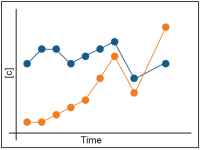
5.8.1 Time series plots

The time series plotA graphic of data collected at regular time intervals, where measured values are indicated on one axis and time indicated on the other. This method is a typical exploratory data analysis technique to evaluate temporal, directional, or stationarity aspects of data (Unified Guidance). provides a graphical view of the raw data. Time is plotted on the x-axis, and the data series observation or observations (for multiple series) are plotted on the y-axis. See Section 5.1.1: Time Series Methods of this document for a complete overview of time series plots.

5.8.2 One-way ANOVA

ANOVAanalysis of variance is a general purpose statistical approach used to compare data from three or more populations (with the data divided into one group/subset per population). Because of its flexibility and generality, ANOVA has utility for spatial analyses (for example, measuring contaminant level differences across multiple wells/sampling points), temporal analyses (for example, evaluating seasonality or temporal correlations across sampling events), as well as diagnostic testing (for example, testing for equal variances or identifying significant spatial variation).

For temporal analysis, the statistical populations to be compared by ANOVAanalysis of variance represent distinct time periods, rather than distinct sampling points as in a spatial analysis. For instance, in cases of apparent seasonality at an individual well, each season (for example, spring or fall) is treated as a distinct population. In order to test for seasonality, each data subset must include representative observations from each distinct season — with a minimum of one sampling event per season collected over a period of at least three years.

When evaluating data sets for temporal patterns due to factors other than seasonality (but which impact a set of wells in common), each sampling event is treated as a separate population. The data are pooledGroundwater samples from more than one sampling point. across sampling points and then grouped/divided by sampling event. The ANOVAone-way analysis of variance then compares the average levels per sampling event to look for differences between events that signify temporal patterns common to the set of wells.

In all parametricA statistical test that depends upon or assumes observations from a particular probability distribution or distributions (Unified Guidance). ANOVAone-way analysis of variance analyses — regardless of how the data are grouped into subsets — the test (parametric F-test) returns an F-ratio statistic and an associated p-valueIn hypothesis testing, the p-value gives an indication of the strength of the evidence against the null hypothesis, with smaller p-values indicating stronger evidence. If the p-value falls below the significance level of the test, the null hypothesis is rejected.. A large F-ratio (and small p-value) indicates that the observed differences between the subsets of data are more than expected based on chance alone, whereas an F-ratio close to one (large p-value) suggests that the differences may be due to random variation.

The Kruskal-Wallis test is a nonparametricStatistical test that does not depend on knowledge of the distribution of the sampled population (Unified Guidance). counterpart to ANOVAone-way analysis of variance that does not require normality of the ANOVA residuals. In this version, ranks of the data are used instead of the observed measurements, and an H-statistic is produced instead of an F-ratio, but the basic thrust of the test is the same. Average ranks are computed for each group being compared. If the differences in rank averages are larger than expected by random variation, the H-statistic will be large (with correspondingly small p-value), indicating a probable difference in the populations.

For diagnostic testing, one-way ANOVAone-way analysis of variance can aid decisions about whether to conduct interwellComparisons between two monitoring wells separated spatially (Unified Guidance). or intrawellComparison of measurements over time at one monitoring well (Unified Guidance). tests by identifying the presence of significant spatial variabilitySpatial variability exists when the distribution or pattern of concentration measurements changes from well location to well location (most typically in the form of differing mean concentrations). Such variation may be natural or synthetic, depending on whether it is caused by natural or artificial factors (Unified Guidance). among a group of sampling points. If the spatial variation is a natural phenomenon, the ANOVA results can help justify use of intrawell groundwater tests. Conversely, the lack of significant spatial variation can point to the use of interwell upgradient-downgradient testing.

Another variation of ANOVAone-way analysis of variance, Levene's test, can also diagnose whether or not multiple populations have similar variances (see Chapter 11.2, Unified Guidance). In Levene’s test, the absolute values of the residuals from a set of wells are treated as the ‘data’ in a standard one-way ANOVA. This tests whether the typical deviations from the meanThe arithmetic average of a sample set that estimates the middle of a statistical distribution (Unified Guidance). of each well differ significantly among the wells, thus signifying differing levels of varianceThe square of the standard deviation (EPA 1989); a measure of how far numbers are separated in a data set. A small variance indicates that numbers in the dataset are clustered close to the mean..

5.8.3 Sample Autocorrelation Function

Autocorrelation is a correlationAn estimate of the degree to which two sets of variables vary together, with no distinction between dependent and independent variables (USEPA 2013b). of a variable, such as a contaminant concentration, with itself over a series of time steps. Autocorrelation may be used to evaluate the frequency of sampling (for example, if subsequent sampling events are correlated, a reduction in sampling frequency may be supported). By computing the first few sample autocorrelation coefficients (ACFs), a plot of ACFs versus the time lags can be prepared; this graph is known as a correlogram (Figure 5-2). The shape of the ACF plot provides information regarding the variability of a given value over time.

A stationaryA distribution whose population characteristics do not change over time or space (Unified Guidance). but nonrandom series will often exhibit a large first-order autocorrelation coefficient, followed by one or two other significant coefficients, with the remaining coefficients tending towards zero. A seasonal series will exhibit a sinusoidal ACFautocorrelation coefficient or function. If the first order autocorrelation coefficient is significant and negative, the series tends to alternate between high and low values. If the series contains a trend, the ACF coefficients will not drop to zero with increasing lag.

5.8.4 Rank von Neumann Ratio Test

The rank von Neumann ratio is used to evaluate seasonality in a data set and is constructed from the sum of differences between the ranks of lag-1 data pairs (for example, data pairs generated by comparison of data collected in a monitoring event to data generated in the previous monitoring event). When these differences are small, the pattern of observations of the data series will be somewhat predictable, and the data series is likely to be autocorrelated. Large differences indicate no autocorrelation. The test is formally conducted by comparing the Rank von Neumann ratio to the tabulated critical points (at a given sample size and desired significance level; see Table 14-1 of Appendix D, Unified Guidance). The Rank von Neumann Ratio test is a nonparametric method.

5.8.5 Seasonality Correlations

If the seasonal pattern in a data series is highly regular, then you can model the data with a sinusoidal function. Moving averages and lag-based differencing (for example, lag-4 for quarterly data, or lag-12 for monthly data) can be used to evaluate the data; see Chapter 14.3.3.1, Unified Guidance. When a significant temporal dependence is identified across a group of wells (for instance, by one-way ANOVAone-way analysis of variance), the adjustment process (moving averages) can be conducted simultaneously for several sets of wells as described in Chapter 14.3.3.2, Unified Guidance.

5.8.6 Seasonal Mann-Kendall Test

The seasonal Mann-Kendall test is a simple modification to the Mann-Kendall test for trend that accounts for seasonal fluctuations. The data series is divided into subsets, with each subset representing the measurements collected during a common sampling event. The standard Mann-Kendall test is performed separately on each subset, with a test statistic performed for each individual subset. The separate, seasonal statistics are subsequently summed to arrive at the overall Mann-Kendall statistic, which is then compared to the critical points of the standard normal distribution.

5.8.7 Temporal Optimization (Cost-Effective Sampling and Iterative Thinning)

Temporal optimization is best represented by the cost-effective sampling method (CES; Ridley et al. 1995; Ridley and McQueen 2005) and later modifications to this approach. In CES, a linear trend is estimated for each chemical-well pair and then classified according to the slope of the apparent trend as well as how much variation exists around the trend. Trends with relatively ‘flat’ slopes (small rates of change) and low variation are recommended for less frequent sampling, while trends with higher slopes or higher degrees of variation are targeted for more frequent sampling. The overriding principle is to (1) sample more frequently at locations where the apparent changes are more dynamic and associated with the greatest statistical uncertainty, and (2) sample less frequently when the trend is changing little and is statistically more certain (that is, less variable).

The second approach is the iterative thinning method (Cameron 2004). Iterative thinning examines whether sampling frequencies can be reduced due to temporal redundancy in the sampling events. This approach identifies redundancy by first estimating a baseline trend using the full data set, after which the trend is repeatedly re-estimated using subsets of the full data to identify the average number of data points needed to accurately reconstruct the baseline. The computations in iterative thinning create a series of ‘what if’ scenarios estimating the nature of the trend that would have been identified if only some of the existing data had been sampled. The overriding principle in iterative thinning is that if a trend can be accurately reconstructed using fewer sampling events, the optimal sampling frequency should be based on this smaller number.

Publication Date: December 2013

Permission is granted to refer to or quote from this publication with the customary acknowledgment of the source (see suggested citation and disclaimer).