5.6 Distributional Tests
Distributional tests are commonly used to evaluate data distribution and to test data for normality. Many commonly applied statistical tests are parametricA statistical test that depends upon or assumes observations from a particular probability distribution or distributions (Unified Guidance). (i.e., they assume that the data follow a specific distribution, that they have a certain shape, and that the data can be described by a few parameters, such as the meanThe arithmetic average of a sample set that estimates the middle of a statistical distribution (Unified Guidance). (a measure of centrality) and standard deviation (a measure of spread).
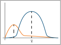
Of the many different types of distributions used in statistics, the most commonly used are the normal distributionSymmetric distribution of data (bell-shaped curve), the most common distribution assumption in statistical analysis (Unified Guidance)., (also known as the bell curve) and distributions that can be transformed to a normal distribution (such as a lognormalA dataset that is not normally distributed (symmetric bell-shaped curve) but that can be transformed using a natural logarithm so that the data set can be evaluated using a normal-theory test (Unified Guidance). distribution). In addition, the gammaA gamma distribution or data set. A parametric unimodal distribution model commonly applied to groundwater data where the data set is left skewed and tied to zero. Very similar to Weibull and lognormal distributions; differences are in their tail behavior, and the gamma density has the second longest tail where its coefficient of variation is less than 1 (Unified Guidance; Gilbert 1987; Silva and Lisboa 2007). and Weibull distributions are used. The normal distribution (bell curve) is well known because of its common use in scholastic grading. This curve plots the frequency of occurrence on the vertical axis and the ordered values of interest, in our case, concentration, on the horizontal axis. If the data follow a normal distribution, most of the data concentrations are near the mean, or average, value and the likelihood of obtaining values away from the mean in either direction tapers off the further the concentration is from the mean.
Appendix A includes several case examples that provide examples of evaluating groundwater data with distributions.
The mathematical model of the normal distribution produces a perfectly smooth, symmetrical, bell-shaped curve. The mean and standard deviation of the data determine the shape of the bell. The mean locates the bell peak on the horizontal axis, and the standard deviation determines the width of the bell. A large standard deviation means that the bell will be broad and flat. A small standard deviation means that the bell will be narrow and skinny (the concentrations in the data set do not deviate much from the mean).
A histogram presents a rough depiction of the data distribution that can be matched with the mathematical model of the normal curve. The histogram, which orders the values, counts the number (frequency) of values within a fixed rangeThe difference between the largest value and smallest value in a dataset (NIST/SEMATECH 2012). of values (a bin) and plots the frequency of values within each bin on the y-axis at the bin’s central value on the x-axis.
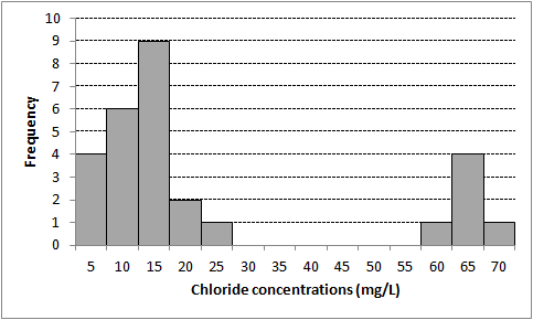
The first task when using a parametric test is to test the underlying assumption of normality. If the data do not produce a nicely shaped bell, for example, if the bell is lopsided or has several peaks, then the underlying mathematical model for the test will not match the data and may produce erroneous results. Other complications might cause the data to appear non-normal, such as outliers, the presence of nondetectsLaboratory analytical result known only to be below the method detection limit (MDL), or reporting limit (RL); see "censored data" (Unified Guidance)., or changes over space or time (nonstationarity). Testing for normality should be conducted in conjunction with tests for outliersValues unusually discrepant from the rest of a series of observations (Unified Guidance). and nonstationarity.
Nondetects are left-censored dataValues that are reported as nondetect. Values known only to be below a threshold value such as the method detection limit or analytical reporting limit (Helsel 2005)., meaning that, below a certain reporting limit the concentrations are not known. Most tests for normality depend on the values at the ends or tails of the ordered data. Too many nondetects in the data set (the Unified Guidance recommends having no more than 10-15% nondetects), can cause problems with the normality tests because the concentrations at the lower tail of the sample distribution are unknown, yet a value is needed for standard normality test to be run. Use caution in substituting values for nondetects, even at low percentages of nondetects. Apply nonparametricStatistical test that does not depend on knowledge of the distribution of the sampled population (Unified Guidance). methods if there is doubt regarding the usability of the data due to the presence of nondetects. See Section 5.7: Managing Nondetects in Statistical Analyses for more information on nondetects.
Outliers are anomalous data found at the tails of data distributions, so their presence may cause problems in testing for normality. If outliers are suspected and a test for normality fails, try removing the suspected outliers and rerunning the test. See Section 5.10: Identification of Outliers for more information on outliers.
Nonstationarity can be an issue with data collected over space or time. The change of concentrations over time or the inconsistency of data over a large area may introduce data that are not in the same distribution. Distribution tests might fail when grouping data sets together even if the original data sets are independently normally distributed. Trend tests or analysis of varianceThe square of the standard deviation (EPA 1989); a measure of how far numbers are separated in a data set. A small variance indicates that numbers in the dataset are clustered close to the mean. (ANOVA) tests should be used if non-stationarityStationarity exists when the population being sampled has a constant mean and variance across time and space (Unified Guidance). is suspected. See Section 3.4.6, Section 5.5, and Section 5.8 for more information on evaluating stationarity.
Many specific methods can test for normality of data distributions, including the goodness-of-fit tests, which compare a chosen distribution with the data set of interest. The following are commonly applied methods:
- Coefficient of Skewness and Variation
- Kolmogorov-Smirnov test
- Graphical assessment of normality (probability plot), probability plots
- Shapiro-Wilk test
- Shapiro-Francia normality test
5.6.1 Coefficients of Skewness and Variation
Because a normal, bell-shaped distribution is symmetric about the mean, normally distributed data will have zero skewnessA measure of asymmetry of a dataset (Unified Guidance).. Therefore, measuring the degree of skewness aids in evaluating data for normality and in evaluating the degree of non-normality. A coefficient of skewness greater than one indicates that the data are not normally distributed. Also, because of the symmetry of the normal curve, the medianThe 50th percentile of an ordered set of samples (Unified Guidance). value will be equal to the mean value. The coefficient of variation (the standard deviation divided by the mean) will also provide some measure of departure from normality. A coefficient of variation greater than one similarly indicates that the data are not normally distributed.
Calculation of the coefficients of skewness and variation can aid in evaluating a data set for normality.
- These methods are not appropriate for data that have been changed by a log transformation.
- Use of a minimum of 8 to 10 values is recommended, a larger data set may be required if data are skewed or contain nondetects
- See Section 5.7 for information on handling nondetects.
- These methods are useful for a quick and easy evaluation of data that will reveal a possible non-normal distribution.
- These methods do not confirm normality, but can provide evidence against normality. Therefore, these methods should be used in conjunction with other tests.
Chapter 10.4, Unified Guidance includes discussion of the coefficient of variation and coefficient of skewness.
5.6.2 Kolmogorov-Smirnov Test
The Kolmogorov-Smirnov test (K-S test) is a common nonparametric goodness-of-fit test that compares the measured data distribution function with the normal distribution function (the mathematical model that generates the normal distribution). Thus, the K-S test compares the graphical curve (in this case, a cumulative fraction plot) of the measured data with that of the normal cumulative fraction plot. The method then calculates maximum distance between the two curves and estimates the p-valueIn hypothesis testing, the p-value gives an indication of the strength of the evidence against the null hypothesis, with smaller p-values indicating stronger evidence. If the p-value falls below the significance level of the test, the null hypothesis is rejected.. A p-value greater than the selected confidence levelDegree of confidence associated with a statistical estimate or test, denoted as (1 – alpha) (Unified Guidance). indicates that the data likely fit a normal distribution. A p-value below the selected confidence level indicates that the data do not fit a normal distribution.
- Goodness of fit tests are used to test the assumption of normality prior to applying other statistical tests.
- Study Question 9: Is the sampling frequency appropriate (temporal optimization)?
The K-S test only applies for continuous distributions, but these distributions are usually expected in environmental systems.
- If the K-S test fails (p-value is less than the selected significance level), try transforming the data and re-testing for normality.
- Use of a minimum of 8 to 10 values is recommended, a larger data set may be required if data are skewed or contain nondetects.
- The K-S test is a robust test that only considers the relative distribution of the data, therefore log-transformation of the data do not negatively affect this test.
- The test is more sensitive around the center of the curve than near the tails.
- The K-S test is not as powerful as the Shapiro-Wilk test.
Chapter 10, Unified Guidance provides information regarding fitting of distributions to data sets
5.6.3 Shapiro-Wilk Test
The Shapiro-Wilk test calculates an SW value. The SW value indicates whether a random sample comes from a normal distribution. If a data set is normally distributed, then a correlationAn estimate of the degree to which two sets of variables vary together, with no distinction between dependent and independent variables (USEPA 2013b). should exist between the ordered data and the normal distribution. Large values of SW indicate a strong correlation while small values of SW are evidence of departure from normally distributed data. This test has performed well in comparison studies with other goodness-of-fit tests.
- Used to test for normality.
- If the SW value exceeds the critical value, the data set is probably normally distributed.
- If the SW is less than the critical value, the data set is not normally distributed. In this case, you may use a data transformation and re-test the transformed data for normality.
Use caution when applying this method to data sets with a large number of nondetects; a larger number of detects will give a better result. For best results, chose a coefficient (α) = 0.10 for very small data sets (n < 10), α = 0.05 for moderately sized data sets (10≤n<20), and α = 0.01 for large data sets (n≥20). This approach is not useful for very large data sets (n>50).
- Because it involves null hypothesisOne of two mutually exclusive statements about the population from which a sample is taken, and is the initial and favored statement, H₀, in hypothesis testing (Unified Guidance). significance testing, if you reject null hypothesis you may conclude that the population is not normally distributed. Rejecting the null hypothesis means that population is not normally distributed, but it does not indicate whether the reason for non-normality is because of a flat-tailed distribution, a skewed distribution, or something else.
- If the null hypothesis is not rejected, you may only conclude that the test failed to show that the population is not normally distributed. In other words, the test can substantiate that the population is not normally distributed, but it cannot prove that the data set is normally distributed.
- The tests are influenced by powerSee "statistical power.". If you have a small sample (n is the number of values), then the test may not have enough power to detect normality in the population. If you have a very large sample, then the test will detect even a trivial deviation from normality.
Chapter 10.5.1, Unified Guidance includes further information and an example for the Shapiro Wilk test.
5.6.4 Shapiro-Francia Normality Test
The Shapiro-Francia test is a simplified version of the Shapiro-Wilk test. The test is generally considered equivalent to Shapiro-Wilk test for large, independent samples. Like the Shapiro-Wilk test, the Shapiro-Francia test calculates an SF statistic to indicate whether a random sample comes from a normal distribution. If a data set is normally distributed, a correlation should exist between the ordered data and the z-scores taken from the normal distribution. Large values of SF indicate a strong correlation while small values of SF are evidence of departure from normally distributed data. The Shapiro-Francia test calculates an “SF” statistic. If the SF statistic exceeds the critical value, the test indicates that data likely fit a normal distribution. If the SF is less than the critical value, the test indicates that the data are not normally distributed. You may subsequently apply a data transformation, and retest for normality.
The Shapiro-Francia method is used to test for normality.
Use caution when applying this method to data sets with a large number of nondetects; a larger number of detected values will give a better result.
- Because it involves null hypothesis significance testing, if you reject null hypothesis you may conclude that the population is not normally distributed. Rejecting the null hypothesis means that population is not normally distributed, but it does not indicate whether the reason for non-normality is because of a flat-tailed distribution, a skewed distribution, or something else.
- If the null hypothesis is not rejected, you may only conclude that the test failed to show that the population is not normally distributed. In other words, the test can substantiate that the population is not normally distributed, but it cannot prove that the data set is normally distributed.
- The tests are influenced by power. If you have a small sample (n is the number of values), then the test may not have enough power to detect normality in the population. If you have a very large sample, then the test will detect even a trivial deviation from normality.
Chapter 10.5.2, Unified Guidance includes information about the Shapiro-Francia test.
Publication Date: December 2013