Each contaminant is made up of elements (for example TCE contains carbon, chlorine, and hydrogen; MTBE contains carbon, oxygen, and hydrogen). Each element within the contaminant has a distinct isotopic ratioThe concentration of the heavy isotope divided by the concentration of the light isotope. (which is the ratio of heavy to light isotopes, such as 13C/12C in carbon within TCE). This ratio is called delta (δ) and is expressed in “per mil” (parts-per-thousand or ‰) relative to some internationally recognized standard. The compound specific isotope analysis (CSIA)Analyzes the relative abundance of various stable isotopes (e.g., ¹³C:¹²C, ²H:¹H). Degradation processes can cause shifts in the relative abundance of stable isotopes of the contaminant; changes in isotopic ratios can be measured. method measures the isotopic ratio precisely relative to a standard, so those differences can be documented and interpreted. The isotopic ratio is initially determined by the natural material of origin and the manufacturing process, but then altered through degradation processes. CSIA can be used to measure degradation of a compound because the isotopic ratio changes as the compound is degraded.
Additional information about atomic structure and the CSIA process is provided in the CSIA Fact Sheet and in Appendix C: Isotopic Chemistry.
Compound specific isotopeTwo atoms with the same number of protons but a different number of neutrons. analysis (CSIA) is used to directly examine individual contaminants to learn both about their original isotopic composition and about any degradation the compound has undergone. CSIA is unique among the EMD tools discussed in this document in that it is not biologically based. This technique also provides unique information concerning chemical fate because the data from CSIA analyses can be used to document contaminant degradation even in the absence of intermediate products or end products. CSIA can provide useful information at sites where there are multiple degradation mechanisms, including both biodegradationA process by which microorganisms transform or alter (through metabolic or enzymatic action) the structure of chemicals introduced into the environment (USEPA 2011). (by one or more pathways) and abiotic degradation (such as in situ chemical oxidation or reduction). For example, CSIA can be used to document contaminant degradation and to distinguish dominant mechanisms at a site where there is reductive dechlorination near the source, co-metabolism down gradient and abiotic degradation across the site. Further, under many conditions, CSIA can be used for forensic purposes to distinguish mixed sources of a single contaminant at a site or to determine the likely original source of a contaminant, such as perchlorate (which has both synthetic and natural origin as described in Case Study A.1). As discussed in the accompanying CSIA Fact Sheet, the utility of CSIA can be further increased for both forensic and environmental fate applications, by analyzing multiple isotopes in a given molecule (for example, both 13C/12C and 37Cl/35Cl in TCE).
CSIA has applications in environmental site assessment and remediation because environmental contaminants are composed of atoms of various elements and most elements have measurable stable isotopesForms of an element that do not undergo radioactive decay at a measureable rate.. Both the forensic identity and the degradation of those contaminants can be traced based on the isotopic composition of one or more of these component elements. Applications of CSIA for evaluating contaminant degradation and distinguishing sources are discussed in more detail below.
Physical processes such as sorption, dilution, diffusion, and volatilization do not significantly change the isotopic ratio of a compound in groundwater. In contrast, the isotopic ratio of an element (for example, 13C/12C) changes in a predictable fashion when bonds between the elements are broken. As the dissolved mass of a contaminant is degraded, the portion of that contaminant that contains a heavy isotope increases. This increase occurs because the bond strength between elements with a heavy isotope (such as the 13C-35Cl bond) is slightly greater than that between elements composed only of light isotopes (12C-35Cl bond). As a result, the reaction rates of molecules with the heavy isotopes are slightly slower, resulting in an enrichment of the parent molecules with a heavy isotope during degradation processes. This “fractionation” process is illustrated in Figure 3-1 for a chemical with a C-Cl bond. Thus, the processes that cause molecular destruction can be isotopically distinguished from physical loss.
Figure 3-1. Example of ¹³C enrichment as biodegradation of a compound with a C-Cl bond proceeds (left to right).
Source: Microseeps, Inc. 2011, used with permission.
CSIA allows measurement of isotopic ratios. Knowledge of the change in isotopic ratios (that is, fractionation or enrichment) allows the data measured through CSIA to be linked to fractionating processes such as biodegradation. As an example, consider the CSIA data collected from multiple measurements of benzene in microcosms. The data produced by those measurements are provided in Figure 3-2. Of course, there is a limit to the precision of CSIA, but CSIA is generally precise enough to measure the changes in the isotopic ratio that biodegradation introduces. The typical precision for carbon CSIA is ± 0.5 ‰, and USEPA recommends a conservative doubling of that range as an indication that biodegradation is occurring (USEPA 2008a). This 2 ‰ range is indicated by the vertical arrow in Figure 3-2. In addition, the initial conditions are at the far right and as degradation proceeds the fraction of benzene remaining decreases, so the relevant data proceeds to the left.
Figure 3-2. Figure showing the isotopic ratio of benzene (expressed as δ¹³C and in units of per mil, or ‰) as the fraction changes.
Source:USEPA 2008a.
CSIA can be used both to measure the extent of degradation and to provide information on the pathway or mechanism of degradation. Multiple degradation processes can often be distinguished based on the extents of fractionation of isotopes of a given element (such as the change in 13C/12C ratio as a function of degradation extent). Mechanisms can also be inferred from the relative extents of fractionation of multiple elements (for example, H and C in MTBE), which can differ significantly when degradation occurs by different mechanisms. This inference is demonstrated in Figure 3-3 for data collected from multiple microcosmA sample that is regarded as a small but representative portion of something larger. In environmental studies microcosm are typically small samples of soil, sediment, or water incubated in enclosed containers under laboratory conditions. studies of MTBE. The data show the difference in the relative extents of fractionation for several mechanisms of MTBE loss. Note that in this case, however, the fractionation of C and H in MTBE by aerobic bacteria shows significant variability, possibly due to different initial reaction mechanisms (Rosell et al. 2012).
Figure 3-3. Plot of the δ²H vs. δ¹³C for MTBE under different experimental conditions. The authors used Δδ = δ – δo, presumably to eliminate variation in the initial isotopic ratio, δo, between the data sets (δ is a measure of isotopic ratio).
Source: Reprinted with permission from Rosell, M., R. Gonzalez-Olmos, T. Rohwerder, K. Rusevova, A. Georgi, F.D. Kopinke, and H.H. Richnow. 2012. Critical evaluation of 2D-CSIA scheme for distinguishing fuel oxygenate degradation reaction mechanisms. Environmental Science & Technology 2012, 46(9) pp 4757-4766. Copyright 2012 American Chemical Society.
CSIA can also be used to investigate both biodegradation and abiotic degradation of contaminants in groundwater. Further, it can be used to measure the contributions of degradation to attenuation versus those of nondegrading mechanisms such as dilution. Some applications of CSIA for examining contaminant loss are provided in the CSIA Fact Sheet. NAVFAC also provides a CSIA tool among its ER Technology Transfer resources. Additional examples are listed in Table 3-1.
In addition to the evaluation of contaminant fate, CSIA is often used in environmental forensicsThe process of distinguishing contaminants from different sources. applications to distinguish between contaminant sources at a site and to identify the most likely source of a contaminant in a specific well. The isotopic ratio of elements in a compound are determined by the source materials that the manufacturers use to make that compound as well as by the manufacturing process used to produce it. The source materials for a specific compound may vary from lot-to-lot or may be very consistent over time. In addition, the manufacturing process may change, therefore a chemical made by Process A may be isotopically distinguished from that made by Process B. Consequently, the isotopic ratios of elements in a chemical may differ over time (due to process or lot variability), even though the chemical is made by the same manufacturer. Initially, researchers did not recognize this variability for chlorinated ethenes, and failed in attempts to use CSIA to identify manufacturers of specific released materials (Beneteau et al. 1999; van Warmerdam et al. 1995). The lot-to-lot variability (and often a lack of good information on the isotopic characteristics of the starting materials), prevents CSIA from specifically identifying a given manufacturer (Shouakar-Stash, Frape, and Drimmie 2003). CSIA can, however, be used to distinguish one source or release of a chlorinated ethene or ethane from another at a given site, particularly when the materials originate from different locations (which can be sampled to determine source isotopic ratios), and then become co-mingled (Smallwood, Philp, and Allen 2002; Slater,2003; Blessing et al. 2009). Additionally, the contribution of each of the multiple sources can be calculated as long as the isotopic composition of each source can be determined and compared to the isotopic composition of the environmental samples.
In some instances, the isotopic ratio of a single element within a contaminant provides enough evidence to forensically distinguish one source from another at a site. For example, the Aviation Plaza data described in Case Study A.3, in which the CSIA of carbon in TCE provided sufficient evidence of multiple sources to justify a membrane interface probe (MIP) investigation which both confirmed the conclusions of the CSIA and provided other valuable information for the conceptual site model. However, results using CSIA for one element are often not as clear as in this example. In many cases, it is desirable to determine the isotopic ratio of multiple elements within a contaminant, rather than just a single element for forensic evaluations. This way, characteristic differences in isotopic ratios among all relevant isotopes can be compared, effectively providing multiple lines of evidence for contaminant differences. One example of this approach is the evaluation of the isotopic ratios of both oxygen (δ18O) and nitrogen (δ15N) in nitrate to distinguish possible sources (atmospheric production, septic systems, manure, and chemical sources such as nitric acid).
Figure 3-4 includes an example of using isotopic data to evaluate nitrate sources with a dual-isotope plot of δ18O and δ15N. The data indicate that the source nitrate was derived from septic systems rather than atmospheric sources (precipitation), nitric acid, or degradation of nitrogen-containing explosives (RDX). The arrow in the figure (denitrification trend line) shows the expected isotopic fractionationSome processes (for example, those which involve breaking chemical bonds) have slightly different rates for different isotopes, leading to a more rapid consumption of one isotope over the other. This characteristic is manifested in a change in the isotopic ratio of the residual compound. of nitrate derived from septic sources if nitrate was biodegrading through denitrification. The data from downgradient wells clearly follow the denitrification trend line.
Figure 3-4. Plot of δ ¹⁸O vs. δ ¹⁵N for nitrate, showing the benefit of using CSIA data from multiple elements in forensics.
Source: Clu-in’s Tech-Trends, Issue 46, February 2010.
In another example, using perchlorate (ClO4-), isotopic ratios of Cl (37Cl/35Cl) and O (18O/16O and 17O/16O) each provide unique evidence concerning the source of this compound in groundwater and soils (Bohlke et al. 2009; Jackson et al. 2010; Sturchio et al. 2012). In this case, synthetic sources from fireworks, flares, and others, can be readily distinguished from natural sources derived from nitrate fertilizers or natural atmospheric processes by comparing data derived from multiple isotopes (see Case Study A1).
Both of the previous cases show data for dissolved contaminants, but CSIA can also be applied to gaseous samples, such as indoor air where vapor intrusion is a suspected source of chlorinated solvent contamination. The basis of the application is presented in Figure 3-5. As indicated in this figure, a comparison of the δ13C value of TCE in groundwater underlying a residence, with the δ13C value of TCE in air within the structure can provide important evidence concerning whether vapor intrusion is the likely contaminant source. Values for δ37Cl can also be used in conjunction with δ13C. As an example, McHugh et al. (2011) (see Case Study A.2) analyzed δ13C in five residences where chlorinated ethenes were present in the indoor air, and in four of those cases, they also measured δ37Cl. In one residences, where only δ13C was measured, the results indicated the contaminant source and no confirmation was needed. In two other residences both δ13C and δ37Cl were analyzed and the contaminant source was found to be consumer products stored within the home. In all three cases, confirmation of these conclusions were not necessary. In the remaining two residences, the CSIA results did not identify a specific source. While CSIA does not always provide clear answers, it shows promise for vapor intrusion applications.
Figure 3-5. Schematic showing reductive dechlorination in the groundwater elevating δ¹³C of the TCE, causing an isotopic ratio distinguishable from that of undegraded TCE in the breathing space.
Source: Microseeps, Inc. 2012, used with permission.
CSIA can be used for monitoring contaminant degradation and for forensic studies. The application of CSIA for monitoring contaminant degradation was previously discussed in Section 3.2.1, with specific examples provided in Figure 3-2 and Figure 3-3. Forensic applications are discussed in the previous section, and specific examples of CSIA at sites contaminated with perchlorate or PCE/TCE are presented in Table 3-1, as well as in the case studies noted. It is beyond the scope of this section to present detailed discussions of each unique application of CSIA for environmental forensics and contaminant biodegradation, however, the following brief summary identifies some common applications and provides references for further information.
For some of the entries in Table 3-1, a full case study is provided in Appendix A. For others, a brief description of the setting, problem, role of CSIA, and the results are provided below.
The M Canal site is an example of the use of CSIA to better understand the in situ fate of PCE and TCE at a site and to use that understanding to develop a remediation strategy that provided significant cost and energy savings. At a facility on the edge of a large river in the Southwest US, a mixture of wastes that included PCE and TCE were released. As part of the remedial effort, a pump and treat system was installed. In order to be protective, the pump and treat system was intensive and involved pumping the contaminated water from the river into the treated land versus from the land to the river. Although costly, the system could not be shut down unless there was sufficient evidence that natural attenuation was occurring. Samples were taken from the treated area and CSIA was performed on the PCE, TCE, cis-DCE, and VC samples. These samples proved that an active pathway to complete dechlorination existed, allowing shutdown of the pump and treat system.
The challenge for this project was to differentiate one LNAPL from another. In an attempt to prove and test the method, seven samples were collected. One of those samples was a duplicate and one was a gasoline sample taken directly from a pump. CSIA–Hydrogen was performed on the samples for 12 compounds. Hydrogen was chosen because there is more range in the δ2H values of petroleum product components than in δ13C, even when considering the higher precision of δ13C measurements (typically ±0.5 ‰) to that of δ2H, typically ±2 ‰ (USEPA 2008a). Two statistical techniques were used to aid in the interpretation: sample pair standard deviation and dissimilarity coefficient (DC).
The DC for the CSIA data was plotted against the DC calculated using the concentrations as shown in Figure 3-6. The difference between the far left group and DEP-6 is obvious. It is less obvious that DEP-4 and DEP-5 are not one group, but the standard deviation for the pairing DEP-4 and DEP-5 is one of the largest standard deviations for any pair. These data indicate that four of the samples, DEP-1, DEP-2, DEP-3 and DEP-7 (a duplicate of sample DEP-1), were from one source. The fresh gasoline sample (DEP-6) was from a second source, and the two remaining samples (DEP-4 and DEP-5) were either from different sources or perhaps contained a combination of two sources. The first two observations were a match to what was known before the test and the duplicate produced excellent results, so the conclusions about DEP-4 and DEP-5 were accepted.
Figure 3-6. 2-D plot of dissimilarity coefficient (DC) for δ²H from CSHIA vs. Molecular DC calculated from the concentrations indicated multiple gasoline sources.
Source: Dr. Yi Wang at ZymaX Forensics Isotope, DPRA Inc., 2012. Used with permission.
At the New Jersey ISCO site, in situ chemical oxidation (ISCO) via potassium permanganate was the chosen remedial strategy for groundwater containing PCE and TCE. There were five ISCO applications. Carbon CSIA data for the chlorinated ethenes were compared pre-treatment and post-treatment for the initial ISCO applications. The CSIA data through four ISCO applications revealed that the oxidant was effectively destroying the chlorinated ethenes, but significant rebound was occurring in the treated area due to delivery complications in complex hydrogeology. Accordingly, hydraulic fracturing was performed prior to the fifth ISCO treatment. The hydraulic fracturing made the final application much more effective and eliminated any rebound in the concentration. The use of CSIA informed the remedial decisions and allowed the project manager to optimize the remedial effectiveness while controlling costs.
Monitored Natural Attenuation (MNA) was the selected remediation strategy for TCE at England AFB. Presumably, the dominant attenuation mechanism was reductive dechlorination. A small amount of ethene was observed, but far less than would be expected if the loss mechanism for TCE was predominantly reductive dechlorination. For many years, the concentrations of TCE, cis-DCE, and VC were all declining. However, during recent monitoring it was discovered the concentrations of cis-DCE and VC increased. These observations led project managers to pursue the use of Carbon CSIA to evaluate the dominant attenuation mechanisms at the site. Three questions were asked: 1) Is the cis-DCE degrading? 2) If vinyl chloride (VC) is observable, is it being degraded? and 3) Has there been any degradation of chlorinated ethenes to anything other than ethene? CSIA was used to answer each of these questions. The CSIA data showed that both cis-DCE and VC at the site were biodegrading and there was evidence of degradation of the chlorinated ethenes to compounds other than ethene such as acetylene or carbon dioxide (Shaw 2010). Without the observation of end products or any assumptions about the degradation mechanism, it was shown that a portion of the TCE present in the initial release has been completely detoxified.
At Naval Air Station (NAS) Pensacola, TCE and sulfuric acid were released into a sandy aquifer. Pump and treat was used from 1986-1997, an ISCO treatment with Fenton’s reagent was performed in 1998-1999, and MNA was used beyond the source area. Biostimulation was investigated as a means to accelerate remediation. The complicated release and remediation history posed challenges for monitoring remediation progress, so CSIA was added to the suite of performance monitoring parameters to help understand the remedial processes. For the biostimulationA remedial technique which provides the electron donor, electron acceptor, and/or nutrients to an existing subsurface microbial community to promote degradation., both changes to chlorinated volatile organic compound concentrations and δ13C data from selected wells were used to evaluate performance. At some wells, the concentration of TCE decreased, but so did the δ13C of the TCE. Further, in some wells, the concentration of cis-DCE rose far beyond what would be expected by the stoichiometric conversion of the TCE previously found in that well. The only explanation for these observations is degradation accompanied by the introduction of residual material.
At the CC site near San Francisco, CA, waste barrels with chlorinated ethenes were stored over a period of years. Chlorinated ethenes leaked from the barrels and eventually entered the groundwater. The contaminants entering the groundwater were from multiple sources and released over a period of several years. Concentration data suggested that a cis-1,2-DCE plume present from the partial reductive dechlorination of the parent compounds (PCE and TCE) was stable, but evidence was required to show that there was an active pathway to complete dechlorination of these compounds to ethene. CSIA of PCE, TCE, and dechlorination intermediate products provided g evidence to show that complete biological reduction of PCE and TCE to ethene occurred at this site.
CSIA data are reported as differences from isotopic standards and discussed in more detail in Section 3.3.1. A discussion of the data quality issues particular to CSIA is presented in Section 3.3.2. Finally, in Section data interpretation is covered explicitly as it relates to the commonly asked questions discussed in Table 2-3.
CSIA is a sensitive technique, which reveals much through the observation of small changes in the isotopic ratio of an element. Because the differences in isotopic ratios are so small, it is more convenient to express the ratios relative to some standard and in “per mil” (parts-per-thousand or ‰) notation. This is accomplished by using the delta formula. The Rstd refers to the isotopic ratio of an internationally agreed upon standard, for example Rstd = 0.01118, is the standard for carbon. The delta formula, in “per mil” is:
Equation 3-1:
where the Rx is the isotopic ratio of sample “x” and δx (called “delta” of sample “x”) is linearly related to the isotopic ratio. Therefore, if the δ(13C) for a TCE sample is “-31 per mil”, (a typical value for undegraded TCE), the 13C/12C in the sample is 31 per mil, or 3.1 percent, lower than in the standard. The only significance of the negative sign is the implication that the isotopic ratio in the sample is less than in the standard.
Additional information about the data reporting is included in Section C.9.
The QA/QC program used for CSIA sampling is largely dependent upon the application. To assist with the correct application of CSIA, USEPA has published A Guide for Assessing Biodegradation and Source Identification of Organic Ground Water Contaminants using Compound Specific Isotope Analysis (USEPA 2008a). This document discusses many of the technical aspects about this technology, including how to best design a CSIA study to address a particular question. Further, NELAC (http://www.nelac-institute.org/index.php) has general standards for sample handling, data manipulation, training, documentation, and reporting, all of which are important issues in acquiring CSIA services but which are not often covered in technical methods or in method specific SOPs. Because there are currently no USEPA-certified CSIA methods, QA/QC procedures should be discussed with the laboratory performing the analysis, the project manager, the applicable regulating authorities, and any other stakeholders prior to the collection of samples for CSIA.
One important issue that has emerged is the use of CSIA values only for sufficiently large contaminant concentrations. Determining a detection limit for CSIA can be complex. Recognizing that background noise can be mistaken as a legitimate detection, the method detection limit (MDL) is intended to be the "the minimum concentration of a an analyze (substance) that can be measured and reported with 99% confidence that the analyte concentration is greater than zero as determined by the procedure set forth in appendix B " (40 CFR 136.2). USEPA recommends (USEPA 2008a):
“…the operational detection limit be defined as that concentration of the compound in the water sample below which the accuracy and reproducibility of the value for δ 13C deteriorate beyond acceptable limits. The criterion for “acceptable limits” depends on the use of the data, and is dependent on the methods and the instruments used.”
To demonstrate how CSIA data can be unreliable at low concentrations, USEPA prepared the graph shown in Figure 3-7. Multiple δ13C analyses were conducted for various concentrations of benzene in water. The standard deviation of the triplicate samples increases as the concentration decreases to less than 0.2 μg/l which is the method detection limit. Below the method detection limit the standard deviation and therefore the precision (indicated by the height of the red bars) becomes unacceptably high. The role of CSIA is not to measure contaminant concentration; enough contaminant mass must be present in a sample to provide reproducible CSIA results.
Figure 3-7. Graph showing decrease in precision of δ¹³C of benzene at low concentrations. Note the very large standard deviation on the analyses as the concentration goes below 0.2 μg/l.
Source: John Wilson, USEPA, data from USEPA 2008a, used with permission.
The exact protocol for a study like the one depicted in Figure 3-7 is beyond the scope of this section, but it is important that the laboratory conducting CSIA analysis carry out similar detection limit studies before the project is initiated so that resources are not spent acting on non-representative data. This detection limit can be thought of as a practical quantitation limit (PQL). Typically there is a small but significant range below the PQL where the results are usable, but do not have the precision and accuracy that is typical of the method. In that case, “J flags” may be used to qualify the peak area. The “J flag” indicates that the measurement is less precise than a measurement at a concentration above the PQL, but still sufficiently accurate and precise to be useful.
The quality control program used for CSIA partially depends on the specific analytical technique used. As such, an overview of the most common isotopic methods is presented below. Note that the analytical equipment used varies among the methods, so the quality control program for one method may be different from the quality control program for another method.
Stable isotopes of an element can be quantified in two basic ways: “bulk” and “compound” specific isotopic ratio analysis. “Bulk” stable isotope analysis measures the isotopic ratio of all compounds in a sample. In CSIA, the compounds are separated and the isotopic ratio of the specific contaminant is measured. This allows CSIA to focus on the individual contaminants. For relatively small elements, such as carbon, chlorine, oxygen, nitrogen, and hydrogen, an isotope ratio mass spectrometer (IRMS) is used to measure the isotopic ratios of small, simple gases such as CO₂ for carbon or H₂ for hydrogen. The bulk method uses an IRMS with an offline process to convert the analyte in the sample to the appropriate gas. This is called “offline sample preparation." The second method uses online sample preparation in which a gas chromatograph (GC) is used to separate compounds of interest prior to isotopic analysis. This instrument is known as a GC-IRMS. It is this online sample preparation that makes CSIA possible.
New techniques are being developed to analyze the stable isotopic ratios of larger elements and those that are not readily converted to a gaseous form. Though they are not ordinarily compound specific, these techniques further extend the range of applications of isotopic analysis. For example, traditional inductively coupled plasma–mass spectrometry (ICP-MS) has been used to determine the concentrations of metals in environmental media and to estimate stable isotopic ratios, but with a relatively large error. The recent development of a multicollector ICP-MS (MC-ICP-MS) allows much more sensitive and precise measurement of the stable isotopic ratios of metals, such as Fe, Pb, Zn, Cu, Mo, and others (Romanek et al. 2010). Each of these techniques is described in more detail in the subsequent subsections.
IRMS with off-line sample preparation - Bulk
This approach has been used for more than 60 years, and involves the initial conversion of the sample of interest to the measured compound, which must be in the gas phase (for example, CO₂ for carbon). The converted sample is then introduced into a dual inlet mass spectrometer simultaneously with the relevant isotopic standard. Depending on the sample preparation method, this analysis is often not compound specific. However, it is still powerful and has been applied for many different elements and compounds. This method can be used for pure compounds or for complex mixtures without pre-separation of individual compounds. However in the case of mixtures, only one isotopic ratio is obtained (e.g., bulk isotopic ratio of δ13C in crude oil) and this approach generates a weighted average of the isotopic composition of all the individual compounds in the mixture. An example of bulk isotopic data is provided in Figure 3-8. This type of data has been used in petroleum exploration for many years.
Figure 3-8. Bulk isotopic analysis of various petroleum sources.
Source: R.P. Philp, unpublished results. Used with permission.
IRMS with off-line sample preparation – analyte isolation
It is possible to isolate the specific contaminant off-line, convert it after isolation, and then use an IRMS to measure the isotopic ratio of the analyte. This method is a form of CSIA and is the most common technique currently used to perform CSIA of Cl and O in perchlorate (for instance, Bohlke et al. 2005; 2009, Gu et al. 2011). The main disadvantage of this technique is that it requires a larger sample mass than similar online techniques. With a contaminant such as perchlorate, which is often present at low concentrations (for example, 10 μg/l) many liters of water may need to be processed to get enough mass for IRMS analysis. This mass is collected by pumping water through special ion exchange cartridges in the field that trap the perchlorate, and then shipping the cartridges to a laboratory for elution and purification of the trapped perchlorate prior to IRMS analysis.
GC-IRMS
An IRMS technique has been developed in the past 25 years that couples a gas chromatograph to an IRMS (GC-IRMS). GC-IRMS makes CSIA possible for many volatile (boiling point 40-180°C) and semi-volatile (boiling point 150-250°C) organic compounds. The ability to separate compounds and then determine the isotopic ratio of multiple separated compounds provided a significant advance in isotopic analysis for environmental applications by allowing stable isotopic ratios to be readily determined for individual compounds in complex mixtures.
In a typical GC-IRMS, all analytes are converted online to light gases prior to introduction into the IRMS for analysis; for example analytes are combusted into CO2 for carbon analysis and pyrolized into H2 for hydrogen analysis. A schematic of a GC-IRMS is provided in Figure 3-9. That particular system is configured to use a purge and trap concentrator to analyze aqueous concentrations of environmental interest and to measure the isotopic ratio of carbon by converting analytes to CO2 and measuring mass 44 (16O12C16O), 45 (16O13C16O and 17O12C16O) and 46 (18O12C16O). Details of how δ is calculated from these three signals are presented in C.7 What is actually measured?.
Figure 3-9. Schematic of a GC-IRMS configured to measure CO₂ from carbon at masses 44, 45, and 46.
Source: Microseeps, Inc. Used with permission.
GC-MS
There are some CSIA studies being conducted using a standard laboratory GC-MS operated in single ion monitoring (SIM) mode. This technique has recently been applied for analysis of Cl isotopes in VOCs and pesticides (Sakaguchi-Soder et al. 2007; Aeppli et al. 2010a). Using this instrument, the mass spectrometer provides both isotopic separation and positive compound identification since the analyte is not converted into a small gas molecule but analyzed by the mass spectrometer directly. As such, for this type of CSIA work, co-elution issues are not as critical.
ICP-MS and MC-ICP-MS
As previously noted, ICP-MS has been used for the analysis of stable isotopic ratios in specific metals, and a newer technique, MC-ICP-MS has been developed to improve the sensitivity and precision of the method. Additional details on stable isotope analysis using techniques and other new approaches can be found in Romanek et al. 2010. Isotope analysis has been used to determine the δ206Pb (presumably in tetra-ethyl lead (TEL) derived from leaded gasoline). In this application, the δ206Pb increases appreciably as an inverse function of the age of the gasoline, from the mid-1960’s to the mid-1980’s. The increasing δ206Pb value is hypothesized to represent a slow shift in the source of the Pb used to produce TEL during this timeframe and is interpreted as linking the lead to leaded-gasoline (Hurst et al. 1996; Murphy and Morrison 2002). These techniques are included to show that a number of different traditional and emerging approaches can be applied for specific forensic evaluation.
The key elements for CSIA report differ somewhat from application to application and target analyte to target analyte. Table 3-2 presents requirements that must be addressed for each application. While an attempt was made to be inclusive, for some applications (for example, perchlorate in groundwater) there are key parameters missing from the table as well as some unnecessary restrictions. It is critical to discuss these issues with the laboratory performing the CSIA measurements prior to the collection of samples. Note that these criteria concur with the guidelines set forth in the USEPA guidance (USEPA 2008a) for samples collected from groundwater.
In most instances, sample collection techniques, preservation methods, and holding times have not specifically been established by regulatory agencies for CSIA analyses. Site managers must discuss sample collection and preservation techniques with the responsible regulator at a site as well as with the analytical laboratory performing the CSIA measurements. In many cases, these laboratories will have SOPs for sample collection and preservation that should be followed to ensure data quality. Moreover, specialized techniques are occasionally required when collecting an analyte for isotopic analysis, as is the case with perchlorate where groundwater is passed through an ion exchange resin column to trap the perchlorate in sufficient quantity for analysis (Bohlke et al. 2009).
As with collection and preservation, there are no USEPA-established holding times for CSIA samples. Often, CSIA analyses will require more time to complete than traditional measurements of contaminant concentration, so using the same holding times for these methods can result in samples being analyzed beyond the recommended holding time for these traditional methods. With proper preservation and storage, and in the absence of any losses to evaporation, sorption, or other physical processes, isotopic ratios in analytes can be stable for several weeks to several months, (USEPA 2008a; Blessing et al. 2008; Hammer et al. 1998). Blessing et al. (2008) reported no substantial fractionation of groundwater containing BTEX or chlorinated hydrocarbons within 4 weeks of sample collection. In the absence of any previously published data on isotope stability for a given compound, recent guidance from USEPA recommends that holding times recommended for the method used to analyze the concentration of the contaminant be used for the CSIA samples as a conservative measure (USEPA 2008a).
To demonstrate how CSIA data can be used to answer the primary questions presented in Table 2.3, examples are considered at each project life cycle stage in the following sections. For the purposes of this discussion, assume CSIA data has been collected from a representative selection of wells throughout each location in the subject sites. After the discussion of how CSIA is used to answer specific questions relevant to CSIA, references for further reading are provided.
B) Are contaminant-degrading microorganisms active?
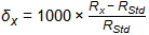
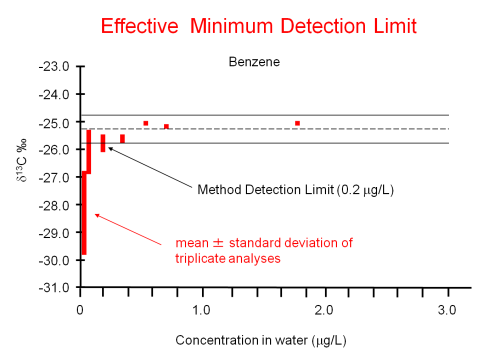
A release at a site contained benzene. After this initial release, contaminant concentrations were observed to decline over time. In addition, sulfate concentrations were lower than background in the core of the plume, indicating sulfate reducing conditions. Reports suggest that benzene degrading organisms are known to exist and be active under sulfate reducing conditions (Lovley et al. 1995). Moreover, the biodegradation of benzene by sulfate reducing strains has been reported to cause isotopic fractionation of carbon in laboratory samples (Mancini et al. 2003). Therefore, to determine if benzene was being degraded (as opposed to diluted), the δ13C values of benzene in groundwater were measured along a flow path downgradient of a suspected source at the site. The resulting δ13C data for each well are displayed in Figure 3-10.
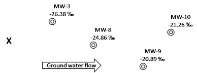
Figure 3-10. Map of an area in the site contaminated with benzene. The δ¹³C of the benzene was measured at each of the wells shown and the results are indicated on the map. Also note that the location of the source is marked with an “X”.
Source: Microseeps, Inc. Used with permission.
The combination of low sulfate concentrations, declining contaminant concentrations, and the increase in δ13C presented in Figure 3-10 suggests that sulfate-reducing benzene degrading microorganisms are active in this area.
D) Is biodegradation occurring?
Benzene Biodegradation
The example for Question B, showing the analysis of δ13C in benzene, answers the question of whether microorganisms are active and also provides clear evidence that biodegradation of benzene is occurring at the site. The increasing values of δ13C in benzene with distance from the source are evidence for biodegradation. With knowledge of groundwater flow rates and the relevant stable isotope enrichment factor (epsilon value) for carbon during benzene biodegradation by sulfate-reducing strains (Mancini et al. 2003), estimates of biodegradation rates can be obtained using stable isotope results. See USEPA guidance (USEPA 2008a) for a detailed description of the method and constraints for determining degradation rates using CSIA results.
TCE Biodegradation
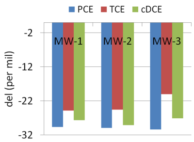
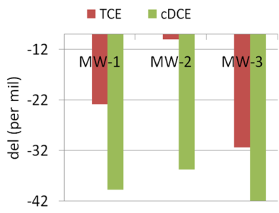
At a site, the primary contaminant is TCE, and it is unclear from the concentration and geochemistry data whether TCE is biodegrading. The TCE was released into a fractured rock aquifer where distance from the source was not necessarily proportional to the time since release. CSIA was performed to see if there was evidence that biodegradation was occurring. An example subset of the results is presented in Table 3-3. In several wells (for example, MW4) the δ13C in TCE was higher, or more positive, than the highest currently published value of δ13C in TCE which is -24.5 ‰ (Aelion et al. 2010). In other locations, (for example MW2) the δ13C for TCE was significantly higher than similar values in the other wells (for example MW1), but not as high as in MW4. Historical records revealed all the TCE in this area was from the same source and the heavier (more positive δ13C) TCE was made more positive by degradation. The observation of TCE with δ13C heavier than the heaviest published literature value for product and of a range of δ13C values that are increasingly heavier than that found near the apparent source (well MW1 with highest residual concentrations) indicate that degradation has been active and that fractionation of δ13C in TCE has occurred or is currently occurring.
These data should be combined with analysis of geochemistry, relevant intermediate products, including cis-DCE, VC and ethene, and appropriate microbial analyses, such as qPCR for DehalococcoidesDehalococcoides is a genus of organohalide-respiring bacteria (for example, bacteria that use chlorinated solvents as metabolic electron acceptors) within the phylum Chloroflexi, in the domain Bacteria, and currently represented by a single species, Dehalococcoides mccartyi (Dhc). This species is the only one known with strains that dechlorinate dichloroethenes (DCEs) and vinyl chloride (VC) to ethene and inorganic chloride. mccartyi (Dhc) to provide additional supporting evidence for TCE biodegradation. The data suggest that the degradation occurring is biodegradation. This is supported by qPCR and the appearance of transformation products. Additionally, the observation of sulfide (as would be expected for respiration through sulfate reduction) and/or the presence of methane concentrations above 1,000 μg/l (as would be expected for methanogenesis) further support the conclusion of biodegradation.
TCE Biodegradation
At another site with TCE contamination, despite decreasing concentrations of TCE, the CSIA values were not significantly different than the heaviest of the published values. There were three potential explanations for this result:
Based on the data, it could not be concluded that biodegradation was occurring at this site. See Aelion et al. 2010; USEPA 2008a; Gray et al. 2002; Song et al. 2002; McLoughlin et al. 2013a; Palau et al. 2010; Morrill et al. 2009.
E) Is the contaminant attenuating abiotically?
At a site, leaded fuel had been released and the fuel additive 1,2-dibromoethane (EDB) was detected significantly above the regulatory MCL of 0.05 μg/L (USEPA 2008b). The EDB concentrations were declining over time, but the mechanism of decline was unclear based on the site data. Analysis of δ13C in EDB collected from several wells on-site was conducted using established methods to evaluate whether degradation could be confirmed based on stable isotopic ratios. The results from the analysis are presented in Table 3-4.
|
Well ID |
Concentration (μg/l) |
δ13C |
|---|---|---|
|
MW5 |
15 |
-18.0 |
|
MW6 |
7.6 |
-10.5 |
|
MW7 |
2.7 |
-4.95 |
|
MW8 |
0.32 |
+11.0 |
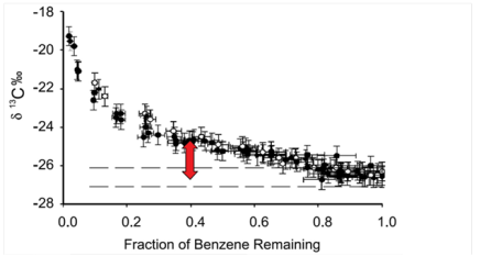
Analysis of δ13C in EDB revealed significant isotope fractionation as a function of distance from the spill, so it was clear that the concentration decline was due at least in part to a degradative process, rather than just dilution or dispersion. The EDB was present in groundwater that was anoxic and has a low oxidation-reduction potential, presumably due to biodegradation of the fuel hydrocarbons. However, EDB degradation has been reported to occur in anoxic environments through both biological processes (Maymo-Gatell et al. 1997) and via abiotic transformation with hydrogen sulfide (H2S) (Schwartzenbach et al. 1985) and iron sulfide (FeS) (USEPA 2008b).
qPCR results showed no degradation capacity despite the application of a wide variety of probes, yet attenuation appeared to be occurring. CSIA results showed that the δ13C of the contaminants were heavier than the heaviest published values. Combined, this strongly suggests abiotic transformation. Further, the fractionation factors (ε values) for carbon during biological and abiotic degradation as shown in Figure 3-11 are such that the very enriched values observed from the field samples strongly suggest abiotic EDB degradation (USEPA 2008b). For additional information on isotope enrichment factors, see Section 3.3.4.1.
For more information on this specific question, see USEPA 2008b; VanStone 2004; Liang et al. 2007; Jeong et al. 2011; Hofstetter et al. 2007; Elsner et al. 2007; Poulson and Naraoaka, 2002).
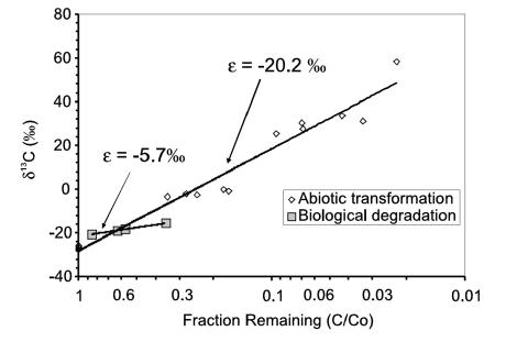
Figure 3-11. δ¹³C of EDB versus the fraction of EDB remaining for a biological study (Henderson et al. 2008) and another study in which the EDB was transformed abiotically.
Source: USEPA 2008b.
F) Are multiple sources contributing to the contamination?
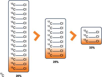
At a site perchlorate was detected in a number of monitoring wells at concentrations, ranging from a few ug/L to several mg/L. Some of the monitoring wells with high concentrations were clearly in an area of the site where propellants were discarded, and the source was easy to identify. However, several other wells with low concentrations of perchlorate were upgradient and sidegradient of this location, and did not have any other anthropogenic contaminants. Based on these data, stable isotope analysis of Cl and O in perchlorate was conducted in the primary plume location and for several of the upgradient and sidegradient wells to determine if multiple sources of perchlorate may be present at the site. The isotope data revealed that the δ18O, δ17O, and δ37Cl values of perchlorate from the primary plume were consistent with values typical for synthetic perchlorate, while the same isotopic ratios for the upgradient and sidegradient wells indicated a secondary low-level source, presumably derived from the past application of natural Chilean nitrate fertilizers (later determined to contain naturally occurring perchlorate) in the region during its past history as agricultural area. An example of the differing isotopic ratios for these sources is provided in Bohlke et al. 2009, and in Case Study A.1 on this topic.
For more information on this specific question, see Bohlke et al. 2005; 2009; Sturchio et al. 2006; 2012, Jackson et al. 2010.
G) If there is a potential for multiple sources, can the sources be distinguished?
Perchlorate
For perchlorate, this question is addressed in Question F. Synthetic and natural sources of this anion can be readily distinguished by stable isotope analysis of Cl and O, although it is much more difficult to discriminate synthetic sources from each other, as values of δ17O and δ37Cl differ very little among synthetic sources (Sturchio et al. 2006).
TCE
For chlorinated solvents, such as TCE, a number of potential situations exist in which multiple sources may be an issue. Most commonly, multiple sources are an issue when one or more sources are contributing to a groundwater plume, or when indoor air is impacted either by vapor intrusion from a plume under the property, or by commercial products brought into a home by the occupants. Both cases were observed at the example site.
Differing δ13C values have been used to discriminate sources of chlorinated ethenes (see Case Study A.3). For the purposes of this example, assume that similar analyses were conducted at one area of the site and showed multiple sources of TCE based on CSIA and supporting chemical concentration and hydrogeological information. Once multiple sources were identified, one of the important questions for wells between the sources was “how much of the contamination is from each source?” CSIA can be used to answer this question, but there are two very different applications of that question. One is for source apportionment in water, the second is for source apportionment in vapor (vapor could be ambient air or soil-gas).
Source Apportionment for a Water Sample
Source apportionment for TCE and other chlorinated solvents is most easily accomplished if biological or abiotic degradation of the parent compound has not occurred. In that case, it can be assumed that the observed δ13C (and δ37Cl values if available) for TCE in a well with mixed sources is just a concentration weighted average of the differing δ values of the individual sources. As an example, in one area of the site where two separate sources were identified, one off-site and one on-site, there was a downgradient well that was contaminated, but the contribution of each source to this contamination was unclear. CSIA was used in an attempt to trace the origin of the contamination and discern what percent of that impact was due to the on-site source and what percent of the impact was due to the off-site source. The site layout is presented in Figure 3-12 and the CSIA results are presented in Table 3-5.
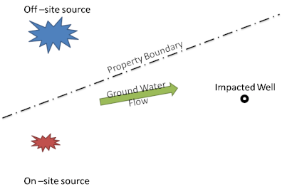
Figure 3-12. The area layout for an example site using CSIA to apportion source contributions.
Source: Microseeps, Inc. Used with permission.
In the impacted well, the δ13C was between the δ13C values of the two sources and the δ37Cl value also was between those of the two sources. In this case, and with no evidence of biological or abiotic degradation of TCE at the site, the contribution of source X is Fx and that of source Y is Fy and the linear relationship for the two sources is as follows:
Equation 3-2:
Equation 3-3:
where δ is δ13C or δ37Cl for TCE from the well in question. Using the data in Table 3-5, the contribution of the off-site well is 80% for carbon. This value is corroborated by a similar calculation indicating the same contributions when chlorine is used.
|
Sample ID |
δ13C |
δ37Cl |
|---|---|---|
|
Off-site source |
-30 |
-2 |
|
On site source |
-25 |
+3 |
|
Impacted Well |
-29 |
-1 |
Source Apportionment for a Vapor Sample
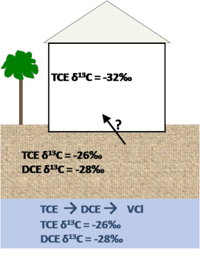
In a home situated above a plume on this site where TCE was being remediated by bio-augmentation and bio-stimulation, TCE was detected in the ambient air at concentrations above the action limit. However, the concentrations were sporadic and the plume shrinking, so it was believed that the source of the contaminant to the indoor air was not vapor intrusion. To better understand this situation, samples were collected from the air in the home and analyzed for δ13C and δ37Cl of the TCE. The TCE was found to be heavier than any published values and such fractionation could only come from degradation. Such degradation is clearly occurring in the treated groundwater plume based on isotope data and supporting parameters, but similar degradation is not expected for any airborne TCE brought into the home via consumer products. This result strongly implicates vapor intrusion from the groundwater plume as the cause of the indoor air concentrations. See Case Study A.2.
For more information on this specific question, see McHugh et al. 2011; Hunkeler et al. 2011; and Bouchard et al. 2008.
K) Are intermediates being degraded?
As a chlorinated solvent is degraded, the first step is conversion to an intermediate product. For example, during reductive dechlorination, TCE typically proceeds through cis-DCE as an initial intermediate product (then VC and finally ethene). At a site, with analysis of δ13C, if the intermediate product of a reaction has the same number of carbon atoms as the starting compound (as is the case for TCE and cis-DCE), and the intermediate product is not degraded (e.g., during cis-DCE stall), the final δ13C of the intermediate product when the starting compound is completely degraded will be identical to the starting δ13C of the original parent compound before any degradation occurred. This relationship is shown in the top panel of Figure 3-13. If the intermediate product is also biodegrading, its δ13C is not limited to that of the parent, as is shown in the bottom panel of Figure 3-13. In cases in which an undegraded sample of the starting compound is not available, the isotopic ratios can be used to infer degradation of the intermediate product (for instance, cis-DCE to VC).
Figure 3-13. δ¹³C of a compound and a nondegrading intermediate compound in the top panel and compound and a degrading intermediate compound in the bottom panel.
Source: Microseeps, Inc. Used with permission.
Example of Intermediates being degraded
At a site where PCE was released, the , δ13C values of PCE and the intermediate products cis-DCE and VC, were measured where the solvent was released to groundwater. In that area, there was an application of a fermentable carbon substrateAny substance that is acted upon by an enzyme. as an electron donorA chemical compound that donates electrons to another compound (based on USEPA 2011). to promote reductive dechlorination. The appearance of the intermediates TCE and cis-DCE were indicative of biological reduction of PCE, but there was no evidence of VC or ethene. CSIA was used to determine if cis-DCE was degrading or persisting, and also to evaluate whether a cis-DCE accumulation (stall) was indicated. This portion of the site was small, and there were only three appropriate ground water wells to sample. The results are shown in Figure 3-14. The results were interpreted by comparing the results for each compound in each well and using the concepts discussed for Figure 3-13. In all three wells, the δ13C in the cis-DCE was heavier (or more positive) than that of the PCE in that well, and this result indicated that the cis-DCE was in fact degrading.
For more information on this specific question, see McLoughlin et al. 2013a; USEPA 2008a.
Figure 3-14. CSIA results showing the δ¹³C of PCE, TCE and cis-DCE.
Source: Microseeps, 2012.Used with permission.
Example of Intermediates not being degraded
At a site where TCE had been released, the concentration of TCE declined over time and the concentration of cis-DCE increased. However, in this area, there were either minimal or no observations of vinyl chloride. In order to see if MNA would be an effective remedy in this area, evidence was needed that the cis-DCE was degrading. Samples were collected and δ13C values of TCE and cis-DCE were measured. The data was collected and is presented in Figure 3-15
Figure 3-15. CSIA results showing the δ¹³C of TCE and cis-DCE.
Source: Microseeps, 2012. Used with permission.
As shown in Figure 3-15, the cis-DCE in each of the wells was significantly lighter in δ13C than the current TCE. However, since there were declining concentrations of TCE and since there was formation of cis-DCE, it can be assumed the TCE was degraded through reductive dechlorination. That degradation presumably resulted in an increase in the δ13C of the TCE, so the criteria that the isotopic ratio of the cis-DCE must be heavier than the current value of the δ13C in the dissolved TCE in each well is conservative. A sample of the undegraded parent TCE was not available to get an accurate, but less conservative measure of degradation. However, as previously noted, there have been several surveys of the δ13C of manufactured TCE. The isotopic ratio of the heaviest or most positive δ13C of TCE in those surveys is -24.5 ‰ (Aelion et al. 2010). It can be considered the upper limit of the δ13C of undegraded TCE. None of the δ13C of the cis-DCE in Figure 3-15 are greater than this limit. Based on this fact, it was determined that cis-DCE degradation was either not occurring at all or not at a rate sufficient to be protective and MNA alone would not be appropriate in this area.
L) Is there evidence of abiotic transformation?
At a site, the primary contaminant was PCE. The impacted aquifer was “aerobic” (that is, it was oxic and supported aerobic respiration) so there had been no degradation of the PCE. Since this area was to be sold within a year, it was necessary to remediate it quickly. In situ chemical oxidation (ISCO) with potassium permanganate (KMnO4) was chosen as the remedial strategy.
However, the regulators at the site were concerned that the injection may simply dilute the contaminant, rather than degrade it. Analysis of δ13C in PCE was conducted in the treatment area to provide evidence of PCE degradation. A previous study (Poulson and Naraoaka, 2002) has shown that an enrichment factor (ε value) for 13C of -13 ‰ should be expected during PCE degradation by ISCO. Since isotopic ratios are not significantly affected by dilution, an increasing value of δ13C in PCE at this site during and after treatment was considered evidence of PCE degradation. Values of δ13C ranging between -4.1 ‰ and -18.7 ‰ were measured. The original δ13C value for the source PCE was not available, However, since the heaviest published isotopic ratio of undegraded PCE is -23.3 ‰, the results were taken as evidence that the PCE was being degraded by the ISCO. The different ranges are shown in Figure 3-16.
Figure 3-16. Range of undegraded product and range of field measurements of δ¹³C of the PCE after ISCO.
Source: Microseeps, Inc. Used with permission.
M) Is biodegradation occurring?
For CSIA, the methods to answer this question are identical to those used for Question D above.
N) What is the rate of biodegradation?
At a site, MTBE had been released and the selected remedy was MNA. While the concentrations were declining, and TBA was present at the site, it was unclear if the TBA was an intermediate or if a co-contaminant that was released with the MTBE. Based on geochemical data (DO, ferrous iron, sulfate, and methane concentrations) it was determined that this location was anoxic and supported anaerobic respiration. As such, the enrichment factor for the biodegradation of MTBE under anaerobic conditions was conservatively estimated to be ε = -12 ‰. An undegraded sample of the MTBE was not available, but the heaviest (most positive) value of δ13C for manufactured MTBE that is reported was used and that was -27.4 ‰. There was an obvious point of release of the MTBE, and the distance from that point to the sampled wells is given in Table 3-6, along with the well ID and the δ13C of the MTBE. The groundwater seepage velocity (v) at this site is 37 meters per year. These values and the data in Table 3-6 were used to estimate the degradation rate using the formula:
Equation 3-4:
Where:
k is the first order rate constant
v is the ground-water seepage velocity
δ0is the initial delta of the contaminant
δtis the delta of the contaminant at time t after the introduction of contaminant
ε is the enrichment factor for the degradation process
d is the distance from the source to the concerned well
|
Well ID |
MTBE δ13C (‰) |
Distance (m) |
k (per year) |
|---|---|---|---|
|
MW-3 |
+6.84 |
9.6 |
11 |
|
MW-8 |
+18.11 |
11.7 |
12 |
Under static conditions, where there is no groundwater flow, other methods exist to calculate rate constants. This is the case for microcosms, but the concentration of contaminant initially placed into the microcosm is known in microcosm studies. In those cases, CSIA is not needed to calculate rates.
For more information on this specific question, see McLoughlin et al. 2013b; Aeppli 2010b; and van Breukelen, Hunkeler, and Volkering 2005.
Q) Are contaminant-degrading microorganisms remaining active?
There is rarely a need to repeat CSIA once a particular question is answered. However, site managers may repeat analyses to see what changes have occurred since a previously established baseline, or as part of a monitoring program designed to use CSIA to establish more definitive answers with less frequent sampling, or to rule out contributions from new sources. An example of the value of repeat analyses is provided in Figure 3-17. MNA was the selected remedy at a site impacted with MTBE, and annual CSIA sampling was used to ensure that remedy was still appropriate. In Figure 3-17, the δ13C of MTBE is plotted against the natural logarithm of the concentration. The dotted lines represent the range of expected δ13C for MTBE in gasoline. In a sealed microcosm, Rayleigh’s law predicts a linear relationship, but at field scale this is not expected because of contaminant flow. Nonetheless, the relationship has been observed multiple times and can be used to assess data from multiple sampling events to confirm that degradation continues, that dilution, dispersion, sorption and volatilization are negligible, and that there are no additional sources contributing to the contaminant mass. Even in cases like the one in Figure 3-17, other than to confirm degradation during active remediation, CSIA is rarely done more often than yearly.
Figure 3-17. Plot of the δ¹³C of MTBE vs. the natural logarithm of the concentration. Data from Table 1 of Kolhatkar et al. (2002).
Source: Adapted from USEPA 2008a.
Additionally, consider the methods to answer this question discussed in Question B above.
S) Are intermediates being degraded?
For CSIA, the methods to answer this question are identical to those used in Question K above.
T) Is there evidence of abiotic transformation?
For CSIA, the methods to answer this question are identical to those used in Question L and Question E above.
U) Is biodegradation occurring?
For CSIA, the methods to answer this question are identical to those used for Question D above.
V) What is the rate of biodegradation?
For CSIA, the methods to answer this question are identical to those used for Question N above.
Some variability of closure requirements exists among states and programs. However, in many situations, EMD data could serve as an additional line of evidence for understanding what processes are important in reducing concentrations and reaching the applicable closure levels. The evidence provided by EMD data would reveal whether biodegradation processes are occurring, have sufficiently proceeded, or are likely to continue.
CSIA provides information on the degradation of a contaminant either since the last time CSIA was used or back to the manufacturing of that contaminant if CSIA was not previously performed at a site. As such, without baseline CSIA data, it is impossible to determine the timeframe over which degradation has occurred or is occurring (i.e., as evidenced by δ values for one of more elements in a contaminant). If CSIA is used to support site closure, particularly as evidence of continuing degradation of a contaminant, measurements must be taken over time. CSIA either needs a baseline or to be complemented with concentrations of short lived terminal electron acceptorsCompounds used by microorganisms to support respiration. In aerobic organisms the terminal electron acceptor is oxygen (O₂). Anaerobic organisms use compounds other than O₂. These include common naturally–occurring compounds such as nitrate (NO₃⁻) or sulfate (SO₄²⁻) or anthropogenic contaminants such as chlorinated ethenes (e.g. perchloroethylene). Atoms from electron acceptors are typically not incorporated into biomolecules made by organisms that reduce these compounds during respiration. (see Appendix D, Question 15) such as ferrous iron or sulfide.
W) Is contaminant degradation likely to continue?
CSIA measures and defines processes that have occurred in the past or are occurring presently. Like most techniques, CSIA is not a predictive tool. However, CSIA can be used to estimate the degradation rate of a compound as discussed in Question K above, and to provide a line of evidence completely independent of the more traditional concentration measurements that biodegradation is occurring at a site. Using multiple CSIA measurements in the same area to establish timeframe, combined with other EMD tools to evaluate microbial populations, this technique can provide useful information for decision making concerning site closure. At a site, rates were measured for TCE biodegradation using CSIA values on multiple occasions and they were similar over time, and compared favorably with available literature rates. In addition, δ13C values were measured for cis-DCE to ensure that this intermediate was continuing to degrade at the site. This result was interpreted as an indication that contaminant degradation was ongoing and the rates were consistent over time.
For more information on this specific question, see USEPA 2005; McLoughlin et al. 2013b; Aeppli 2010b; van Breukelen, Hunkeler, and Volkering 2005.
X) Are intermediates being degraded?
For CSIA, the methods to answer this question are identical to those discussed in Question K above. For closure, review the stable isotopic ratios of intermediate products (such as cis-DCE at TCE or PCE sites) even when traditional concentration measurements cannot detect downstream intermediates such as vinyl chloride.
Y) Is biodegradation occurring?
For CSIA, the methods to answer this question are identical to those discussed in Question D above.
Z) What is the rate of biodegradation?
For CSIA, the methods to answer this question are identical to those discussed Question N above.
CSIA is a powerful tool that allows site managers to evaluate contaminant fate and transport independently of traditional concentration measurements. This tool also can provide valuable forensic information concerning the original source of contaminants in groundwater, soils, or air. However, as with any technique, be aware of both the advantages and the limitations of this technique.
Because of slight differences in bond energy, biodegradation and chemical degradation occur slightly more rapidly for molecules containing only elements with light isotopes compared to those with both light and heavy isotopes. This difference leads to an isotopic enrichment in the parent molecule, and the strength of this enrichment is termed the enrichment factor (ε), as previously described in Figure 3-13 and accompanying text. Both in concept and in practice, enrichment factors are useful and accurate. The following lists points out important issues that should be considered when using enrichment factors.
Despite some limitations, enrichment factors can provide important information concerning the fate of an environmental contaminant. They can be used to discriminate degradation mechanisms and aid in monitoring the effectiveness of a remediation approach. Moreover, enrichment factors can be used with site specific CSIA data to calculate degradation rates for simple mechanisms (USEPA 2008b) and can help constrain the rates in complex mechanisms such as those involving intermediate products (van Breukelen, Hunkeler, and Volkering 2005) or even be combined with other techniques allowing for determination of location-specific rate constants (Aeppli et al. 2010b).
CSIA examines one environmental medium at a time, but the isotopic ratios of contaminant mass are controlled by what occurs in the dissolved phase as well as the non-aqueous phase and the vapor phase. (Morrill et al. 2009; ISCO site; NAS Pensacola site).
While continual processes build upon previous isotopic effects, once an isotopic effect occurs, it remains. As such, CSIA does not necessarily represent recent history unless certain precautions are taken. It may be desirable to couple CSIA measurements with a time sensitive indicator such as dissolved hydrogen or to use multiple sampling events to evaluate temporal evolution (McLoughlin et al. 2013a).
Heterogeneity creates substantial variation across a site. Degradation occurring in one area may not be occurring in another. The primary source influencing one portion of a plume may be different than the primary source influencing another portion of the plume. Because CSIA is relatively affordable, it can and should be done at multiple points across a site to account for variability (Courbet et al. 2011; Gaganis, 2005; Song et al. 2002), since the observations at one location may not reflect the rest of the site.
While CSIA data provide useful forensic evidence, several issues must be considered before using the method in forensic investigations:
Further reading specific to CSIA is provided in Appendix F.